| Issue |
Aquat. Living Resour.
Volume 33, 2020
|
|
|---|---|---|
| Article Number | 10 | |
| Number of page(s) | 15 | |
| DOI | https://doi.org/10.1051/alr/2020010 | |
| Published online | 04 September 2020 | |
Research Article
The population dynamics of the red porgy Pagrus pagrus along southern Brazil, before its fishery collapse in the 1980s: a baseline study
1
Laboratório de Recursos Pesqueiros Demersais, Instituto de Oceanografia, Universidade Federal do Rio Grande, FURG. Av. Itália, km 8, CEP: 96203-000, Rio Grande, RS, Brazil
2
Graduate Program in Biological Oceanography, Instituto de Oceanografia, Universidade Federal do Rio Grande, FURG. Av. Itália, km 8, CEP: 96203-000, 16 Rio Grande, RS, Brazil
* Corresponding author: This email address is being protected from spambots. You need JavaScript enabled to view it.
Handling Editor: Verena Trenkel
Received:
30
January
2020
Accepted:
14
July
2020
Abstract
The intense exploitation since 1972 of the formerly only slightly exploited protogynous hermaphroditic fish Pagrus pagrus (L.) in southern Brazil has led in less than a decade to the collapse of the fishery, with no recovery four decades later. In this study we analized the age structure, growth, reproduction and mortality of the species were studied based on samples collected from 1976 to 1985 to provide a baseline before the onset of overexploitation. Maximum estimated ages were 21 and 26 years based on scale and otolith readings, respectively. Mean total length (TL) at age did not differ between males and females, while hermaphrodites were smaller. The von Bertalanffy growth coefficients for all fish (immature, females, hermaphrodites and males) were L∞ = 447 mm, k = 0.204 and t0 = −1.134 yr. Change in growth was observed during the study period. Females were dominant at all sizes, hermaphrodites were only present up to intermediate sizes, and males, despite being infrequent at small sizes, made up over 40% among the larger specimen (TL > 400 mm). Spawning took place mainly in late spring and condition factors were lower after spawning. Natural mortality was estimated as M = 0.173 yr−1 based on the von Bertalanffy growth parameters. Total mortality (Z) and exploitation rate (E) estimated from catch curves of fully recruited red porgies aged five to ten years increased from 0.24 yr−1 and 28% before 1973 to 0.49 yr−1 and 63% in the following years. Two distinct scale and otolith patterns, one with well-marked annuli and another with faint or absent annuli, suggested that the red porgy stock off southern Brazil might not be homogeneous and may include subpopulations that do not fully mix.
Key words: Age determination / growth / mortality / reproduction / size and age structure / red porgy stock
Deceased
© EDP Sciences 2020
1 Introduction
The red porgy Pagrus pagrus is a sublittoral demersal fish species with a wide distribution on the subtropical and warm temperate continental shelves of the Mediterranean sea, in the eastern Atlantic from the British Isles to Angola, and in the western Atlantic from the latitude of New York to that of Argentina (Ball et al., 2007). It is a relatively sedentary species that has a patchy distribution over irregular and low profile hard bottoms (Manooch and Hassler, 1978). The species supports commercial and recreational fisheries throughout its distribution range. During recent decades, more than half of recorded catches came from the southwestern Atlantic (FAO, 2018). Since the 1950s, landings in Argentina peaked at 15 365 tons in the 1980s and decreased to less than 1000 tons in the late 1990s before recovering to over 7000 tons in 2009, and falling again to around 4000 in recent years (Lagos et al., 2009; MAGyP, 2017). In Uruguay, landings never exceeded a few hundred tons (CTMFM, 2018). In southern Brazil, until 1972, red porgy was a bycatch in the inshore bottom trawl fishery. In an exploratory bottom trawl fishing survey carried out in 1972, a large concentration of red porgy was detected between 50–80 m depths near the Brazil − Uruguay border (Yesaki and Barcellos, 1974). In the winter of 1973, a large number of trawlers shifted from shallow coastal waters to the new fishing grounds and fished 5898 tons of red porgy. Recorded landings decreased rapidly in the 1980s to 240 tons in most recent years (Ibama/Ceperg, 2011; MPA-FURG, 2018).
Different aspects of the biology, population dynamics, stock structure, and fisheries of red porgy have been studied in Brazil and Argentina because of the importance of the species in the southwestern Atlantic (Cotrina, 1977; Cotrina and Christiansen, 1994; Cotrina and Raimondo, 1997; Lagos et al., 2009; García et al., 2011; García and Déspos, 2015; Militelli et al., 2017; Haimovici et al., 1996; Haimovici, 1998; Capitoli and Haimovici, 1993; Ávila-da-Silva, 1996; Costa et al., 1997; Ávila-da-Silva and Haimovici, 2006; Porrini et al., 2015; Soares et al., 2018; Kikuchi, 2019).
The red porgy is a sequential protogynous fish. Three types of gonadal developments have been described: (i) gonochoric males, also referred to as primary males, where immature fish develop the testicular tissue and the ovarian tissue degenerates before sexual maturity; (ii) protogynous hermaphrodites, where immature fish develop the ovarian zone of the gonads and after single or possibly repeated spawning, change sex and function as males, which is referred to as the secondary male type (Fostier et al., 2000); and (iii) females, where immature fish develop the ovarian tissue and never change sex.
In 1976, the University of Rio Grande initiated a sampling program of the demersal fish resources landed by the industrial fleet in Rio Grande (Haimovici, 1987). The aim of this program was to study the population dynamics of the main species caught by the trawl fishery, including red porgy between 1976 and 1985. In this paper, we analyzed some aspects of the population dynamics of red porgy along southern Brazil in the late 1970s and early 1980s including age estimation and growth, annual reproductive cycle, size and age structure, stock identification through scale patterns, mortality and exploitation rates. This paper is expected to be used as a baseline for future studies on the population dynamics of the unrecovered stock of the species in southern Brazil.
2 Material and methods
2.1 Sampling and data collection
Data on the size, sex and biology of red porgy were obtained from a regular sampling program of industrial fisheries landings in Rio Grande between 1976 and 1985 and occasional bottom trawl surveys along southern Brazil (Haimovici, 1987; Haimovici et al., 1996) (Fig. 1).
During dock sampling, total length (TL), measured from the tip of the snout to the midpoint of the upper and lower limbs of the caudal fin, was recorded in 1 cm interval classes to analyze the length composition. Specimens selected for age determination and reproductive cycle studies were measured in millimeters, weighed in grams (TW) and sexed (undetermined, male, female or hermaphrodite). Maturity stage and gonad weight (GW, g) were recorded. For age determination, scales from behind the pectoral fin insertion were collected, cleaned and mounted between glass slides. Most scales from this region are large, symmetrical and the proportion of regenerated scales is low. The linear relationship between the total length and the mean central radius of the scales of 116 individuals measuring 160 to 420 mm was calculated. Sagittal otoliths of a small sample (n = 101) were collected for comparison of estimated ages from scales and otoliths. Otoliths were transversally sectioned (0.2 − 0.3 mm) through the nucleus with a low speed rotary saw and examined under reflected light.
In addition to noting total landings for each sampled fishing boat, between 91 and 360 specimens were necessary to ensure 95% confidence intervals of 10 and 5 mm, respectively (Haimovici, 1987).
 |
Fig. 1 Sampling sites for Pagrus pagrus landed between 1976 and 1985 by pair trawlers (triangles), otter board trawlers (circles) and handliners (squares) from the industrial fleet of Rio Grande, RS, Brazil. |
2.2 Age determination and validation
Scales that had previously been cleaned in a 1% thymol water solution were mounted dry between two glass slides and examined under a binocular microscope. After several preliminary readings, two readers counted the rings independently. In cases of disagreement, a third joint reading was carried out. If the disagreement persisted, the individual was excluded from the age sample. To estimate maximum age, thin sections of the otoliths were prepared so that the alternate opaque and translucent bands could be counted even for the older specimens that had crowded rings at the edge of their scales.
The periodicity of ring formation was evaluated by analyzing the distances between the last fully formed ring and the anterior border of the scales, which were measured on the screen of a microfilm projector. For each aged specimen, a marginal increment index (MI) was calculated as follows:
where R is the distance from the focus to the anterior margin of the scale, and Rn–1 and Rn are the distances to the second to last and last rings.
2.3 Weight–length relationships
There is no known distinctive character between juvenile females which will change sex at some time and those which will remain female throughout their lifetime. As the species is hermaphrodite, it is impossible to known whether the size, weight and age of an individual at the time of sampling resulted from growth accomplished with the observed sex or with the other sex. Therefore, possible differences in weight–length relationships are difficult to interpret and only the relationship of all fish independent of sex is of practical interest. Therefore, a single relationship between weight and length was described for all specimens fitting the model TW = a TLb .
2.4 Allometric condition factor (K)
Allometric condition factors (K) (Heincke, 1908; Le-Cren, 1951) were calculated as follows:
where b is the coefficient of the weight–length relationship obtained for each period.
2.5 Growth
Back-calculated lengths-at-age were computed using the proportional scale hypothesis (Francis, 1990) with the Fraser-Lee formula: where TL is total length in mm at the time of capture, TLi is the length at the formation of the ith ring, Ri are distances between the focus and each age ring and c is the intercept of the linear relationship between scales radius (R, mm) and fish length (TL, mm).
Length-at-age data were fitted by a nonlinear iterative quasi-Newton algorithm to the von Bertalanffy growth model (VBGM), which is expressed as TLt = TL∞ (1 − e(−k(t−t0))) where TLt is length (mm) at age t (years), L∞ asymptotic length (mm), k the instantaneous growth coefficient and t0 the theoretical age at zero length (years). A likelihood-ratio test (α = 0.05) was used to compare mean length-at-age and the von Bertalanffy growth model parameters between males and females (Aubone and Wöhler, 2000; Cerrato, 1990).
2.6 Reproductive cycle
Specimens were classified from macroscopic examination as hermaphrodites when both testicular and ovarian tissues were present in the gonads, and as males or females when all or most of the tissue was testicular or ovarian, respectively.
Maturity stages were determined macroscopically with a seven-point scale: (1) virginal immature, (2) developing virginal, (3) developing, (4) advanced development, (5) running, (6) partly spent, and (7) recovering (Holden and Raitt, 1975) that was used as a standard scale for the sampling of demersal fishes landed in Rio Grande (Haimovici and Cousin, 1989). Although other scales are more adequate for red porgy (see Militelli et al., 2017), the one used here discriminates between immature, maturing, mature, partly spent and resting stages.
The seasonality of reproduction was analyzed from changes in the monthly proportion of mature specimens (stages 3, 4, 5 and 6) and average gonadosomatic indices (GSI) calculated as GSI = 100 (GW / TW) (Wootton, 1998), where GW is gonad weight in grams.
2.7 Age composition and mortality
Age compositions in the landings of pair and otter trawlers and gill net fishing boats were calculated by combining age-length keys with length frequencies for the years 1976 to 1985.
Instantaneous total mortality (Z) was estimated from the age composition as the slope of the catch curve (Ricker, 1975). The 95% confidence interval of Z was calculated by bootstrapping (Hammer et al., 2001).
Instantaneous natural mortality was calculated with the empirical estimator M = 4.118. K0.73 L∞−0.33 (Then et al., 2015). M inferred from the von Bertalanffy growth model coefficients, rather than from the observed longevity, was preferred because it is less influenced by the subjectivity of age estimation for very old fish or their absence on the fishing grounds for which the samples were collected.
3 Results
Overall, between 1976 and 1985, 22491 red porgies were measured from the landings of otter board trawlers (43), pair trawlers (18) and handline fishing boats (6) (Tab. 1). During the sampled fishing trips, otter board trawlers fished mostly in the cold season at depths from 50 to 120 m, pair trawlers fished year-round mostly at depths shallower than 50 m, and handliners fished on rough bottoms at depths between 70 and 80 m in winter and spring. Red porgies made up 67% of total landed weight of the sampled catches of handliners, 23% of otter board trawlers, and 6% of pair trawlers.
Number of sampled fishing trips, number of measured specimens and mean total length of Pagrus pagrus landed by handliners, pair trawlers and otter board trawlers in southern Brazil between 1976 and 1985.
3.1 Scale patterns
The scales of red porgy are ctenoid and subrectangular in shape with 7 to 12 radii in the anterior field. The circuli follow approximately the shape of the scales. The growth rings, or annuli, appear as discontinuities in the circuli.
In most samples, the growth rings on the scales were classified as “well-marked” and most specimens were easily aged. In some samples, many specimens had “faint or absent” rings on the scales (Fig. 2). Each specimen showed the same pattern in all its non-regenerated scales. Specimens with well-marked, faint or absent rings on scales were found in both sexes and for the entire size range. The overall percentage of specimens with well-marked rings was 64.9% (n = 3696); this percentage was much lower in the last quarter of the year (October–December) (32%) compared to the other quarters (Fig. 3).
 |
Fig. 2 Otolith section and scales of Pagrus pagrus fished along Southern Brazil with “well-marked” annuli (a, 9 years old 450 mm TL) and faint or absent annuli (b, unaged, 450 mm TL). Scale bar 1 mm. Black lines indicate annuli; black circle indicate the focus; arrow indicate the circuli discontinuity; and the white dashed line indicates the central radius. |
 |
Fig. 3 Quarterly proportion of growth rings classified as “well-marked” in scales of Pagrus pagrus sampled in southern Brazil between 1976 and 1985. |
3.2 Weight–length relationship and conditions
The weight–length relationships for fishes between 180 and 500 mm was TW = 1.735 10−5 TL 2.9790 (n = 2963; R2= 0.9814) (Fig. 4).
 |
Fig. 4 Weight–length relationship for pooled sexes of Pagrus pagrus sampled in southern Brazil between 1976 and 1985 (n = 2963). Continuous line indicates the regression line (W = 1.735 × 10⁻⁵ × TL2.9790; R2= 0.9814). |
3.3 Age validation
The annual formation of rings was validated analyzing the monthly variation of the proportion of specimens aged 2 to 6 years that had the last ring on the border of the scale (n = 2692). The bimonthly changes and the frequency distribution of the marginal increments (MI) of the scales (0.2 mm intervals) of 309 red porgies with two and three rings in their scales were also analyzed. The monthly proportion of specimens with rings on the border of the scale was over 40% between December and February and less than 5% from June to September (Fig. 5). The thinnest marginal increments occurred between November and February, while MIs over 0.4 were more frequent from May to October (Fig. 6). These observations suggested that rings on the scales form annually in winter and early spring and become evident on the border of the scales when growth accelerates in late spring and early summer.
The largest number of rings (annuli) on scales was 21, and the largest number of alternate opaque and translucent bands in sectioned otoliths was 26 (Fig. 7). The comparison of the annuli readings was possible for 89 red porgies that were aged using both scales and otoliths. Age determinations agreed for 53% of specimens and differed by one year in another 40% (Tab. 2). The correspondence was considered overall good, showing that both structures are adequate for age determinations. However, for older fish, age determination on scales is less reliable because of the crowding of the rings at the scale border. For example, a specimen with 12 rings on the scale had 19 opaque bands in its otolith.
 |
Fig. 5 Monthly proportion of Pagrus pagrus sampled in southern Brazil aged 2 to 6 with the annuli in the border of the scales (n = 2692). Vertical bars represent 95% confidence intervals. |
 |
Fig. 6 Bimonthly frequency distributions of marginal increments (MI) with two and three rings in the scales of Pagrus pagrus from southern Brazil. |
 |
Fig. 7 Thin transverse section of sagitta otolith of a 26+ years old Pagrus pagrus fished in 1976 along southern Brazil. Scale bar 0.5 mm. White circles indicate the annuli; black circles indicate the focus. |
Differences between the readings of annual growth marks in otoliths and scales of Pagrus pagrus.
3.4 Growth
Mean total length of males, females, and hermaphrodites was calculated for all age classes with more than 10 specimens. Kruskal–Wallis tests did not show any significant differences between males and females except at age five and temporary hermaphrodites were smaller than both males or females at ages two and three (Tab. 3).
The linear relationship between total length and the mean radius of the scales of 116 specimens measuring 160 to 420 mm was calculated as TL = 4.37 R − 92.225; R2 = 0.957. The back-calculated TL at the formation of the annuli on the scales at each age for 1041 males, females, hermaphrodites and unsexed red porgy samples from 1976 to 1978 are shown in Table 4.
Mean TL at age between 1976 and 1985 did not show any trend, therefore the von Bertalanffy growth curves by sex were calculated using data pooled across the sampling period (Fig. 8).
The difference between mean total length of the catch and mean back-calculated length using the scales showed that bottom trawls fished selectively the larger red porgies at ages one and two, and only specimens aged three and older were fully retained by the bottom trawls (Tab. 4). Back-calculated TL at ages 1 and 2 better represent the growth of specimens not fully recruited to the fishing gears. Therefore, the von Bertalanffy model parameters (Tab. 5) were calculated using the interpolated TL at age 1 and 2 from the mean back-calculated TL at age (Tab. 4) and the mean TL observed in each age class from 3 to 15 (Tab. 3).
The calculated parameters for the pooled sexes, including unsexed and hermaphrodites individuals, were L∞ = 447 mm, k = 0.204 and t0 = −1.134 yr; the asymptotic weight using the estimated weight-length equation was W∞ = 1 363 g.
Mean total length at age (TL), the number of specimens (n) and 95% confidence intervals (Cl) for male, female and hermaphrodites and pooled sexes of Pagrus pargus from southern Brazil sampled between 1976 and 1985. The results of the Kruskal–Wallis test between sexes by age are shown in the right column. The pooled sexes number includes non-sexed specimens.
Back-calculated total length (mm) at age of pooled sexes of Pagrus pagrus fished from 1976 to 1978 along southern Brazil.
 |
Fig. 8 Mean total length of Pagrus pagrus sampled in southern Brazil at ages 1 to 11 in the years 1976 to 1985 (n = 4 274). |
Von Bertalanffy's growth parameters and their respective confidence intervals (CI = 0.05) for Pagrus pagrus fished off southern Brazil.
3.5 Reproductive seasonality and fish condition factor
Average total length-at-maturity and age-at-maturity were not estimated because of the small number of young red porgies sampled in October and November. However, it was observed that few specimens were mature under 270 mm and only six among the 14 specimens at age three (43%) were maturing or mature. Therefore, the annual cycle of gonadal maturation and the condition factor of adult red porgies were calculated using only specimens over 270 mm. The highest proportions of specimens with developing to partly spent gonads (stages 3 to 6) were from October (52%) to December (62%) for males and between October (68%) and November (85%) for females, later decreasing from December to April (<25%) (Fig. 9).
The gonadosomatic index for both sexes increased sharply in October and attained a maximum value in November (GSI females = 3.70; GSI males = 3.08) before decreasing in December and remaining low from February to September (Fig. 9). It was concluded, that in southern Brazil most spawning occurred in spring. However, maturing and mature females were observed until early autumn.
The monthly average K of red porgies larger than 270 mm was lower between August and January compared to February to July (Fig 10).
 |
Fig. 9 Mean monthly gonadosomatic index (line) and percent of maturing and mature macroscopic stages of male (a) and female (b) Pagrus pagrus over 270 mm total length from southern Brazil. Vertical bars represent 95% confidence intervals. |
 |
Fig. 10 Monthly average of condition factor for pooled sexes of Pagrus pagrus between 270 and 450 mm TL (n = 2495) fished along southern Brazil. Vertical bar represents 95% confidence intervals. |
3.6 Sex ratios
We analyzed the gonads of 2907 red porgies, among which 6.1% were juveniles that could not be sexed: 9.2% were hermaphrodites, 53.2% were females, and 31.5% were males. Most specimens smaller than 180 mm had filiform gonads that could not be macroscopically sexed; hermaphrodites were more frequent between 210 and 300 mm, but some attained over 400 mm; and female was the most frequent sex for fish over 240 mm. Among the 2228 specimens aged, the proportion of males gradually increased with size and reached over 35% of the fish over 300 mm and near 50% among the larger sizes (Fig. 11a). Hermaphrodites were more frequent at the younger ages and became infrequent among fishes over 6 yrs., females were dominant at all ages over 2 yrs. and the proportion of males increased with age and made up over 40% of the red porgies aged over 8 yrs. (Fig. 11b).
 |
Fig. 11 Sex ratio by (a) total length classes of 30 mm intervals (n = 2907) and (b) by age classes (n = 2228) of Pagrus pagrus sampled in Rio Grande from 1976 to 1985. |
3.7 Length and age compositions
Length and age frequencies for each fishing gear and year from 1976 to 1985 are shown in Figure 12. Age frequencies were calculated by combining the length frequency with the length-age key (Tab. 6). Because no changes in length-at-age were observed during the study period (Fig. 8), a common age-length key was used to reduce random errors, particularly among the older red porgies.
Red porgies landed by otter board trawlers between 1976 and 1984 included few small specimens, and the length frequency distributions were mostly unimodal with a mean TL of 331.4 mm. Age compositions were unimodal with ages three to five as the most frequent age classes (Fig. 12).
The catch of pair trawlers between 1976 and 1985 included both small and large red porgies measuring on average 334.4 mm TL. Annual length frequencies were multimodal and variable between years. Most age compositions were also multimodal, in 1976 the most frequent age was seven years, in the following years it ranged from two to five years, and a slight pattern of decrease in the frequency of the older individuals was observed (Fig. 12).
Handliners landed mid-sized and large specimens over 500 mm, with a mean of 370.8 mm. Length frequency distributions were unimodal in 1983 and bimodal in 1984. Age compositions were mostly unimodal and fishes in the age class seven years were the most abundant (Fig. 12).
Otter trawlers targeted concentrations of large red porgy. Therefore, the length compositions in their landings were considered to provide the most representative samples of the age structure of the adult fraction of the stock for total mortality estimates.
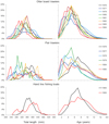 |
Fig. 12 Relative length and age composition in the landings of Pagrus pagrus fished along southern Brazil between 1976 and 1985 by pair trawlers, otter board trawlers, and handliners. |
Length–age key of Pagrus pagrus from southern Brazil sampled between 1976 and 1985. TL total length in mm.
3.8 Mortality and exploitation rate
The instantaneous natural mortality coefficient was calculated using the estimated von Bertalanffy growth coefficients (k = 0.204 and L∞ = 447) as M = 0.173. Further, annual instantaneous total mortality coefficients for the period 1976 to 1984 were calculated using annual catch curves for ages 5 to 10 and represented the mean total mortality suffered by red porgies fully recruited to the bottom trawl fishery (Ricker, 1975). The 5 to 10 years age range was a compromise between including a wide range of ages for which data were available, and minimizing the violation of the assumption of constant fishing and natural mortality in the years represented in the catch curves (Ricker, 1975). The Z estimates were averaged for two periods, representing before and after the intensification of fishing along southern Brazil. The first period included Z estimates from 1976 to 1979 with mean Z = 0.25 yr−1 (0.20 to 0.29 yr−1) and an exploitation rate (E = F / (F + M) x100) of 28% (13 to 41%). The second period included annual estimates from 1980 to 1984 in which the mean Z was nearly doubled to 0.49 yr−1 (0.42 to 0.64 yr−1) and mean E was more than doubled to 63% (59 to 73%) (Fig. 13). Estimates for the first period included cohorts born between 1969 and 1974, which were only marginally affected by the rapid expansion of fishing in the second half of 1973. In contrast, the second period included cohorts born between 1975 and 1979, which were affected by intense fishing. Comparing mean total morality values for the two periods, total mortality of red porgies aged over 5 years increased by 100% and exploitation rate by 126% because of the intensification of fishing in 1973.
 |
Fig. 13 Annual total instantaneous mortality coefficient Z (upper panel) and exploitation rate E (lower panel) of Pagrus pagrus fished in southern Brazil between 1976 and 1984. Vertical bars represent 95% bootstrap confidence intervals. |
4 Discussion
The red porgy Pagrus pagrus has a large distribution range, and its biology, population dynamics, and fisheries aspects have been studied in different regions of the western and eastern Atlantic Ocean and Mediterranean Sea. The results found herein reveal both common and contrasting aspects of red porgy population dynamics in southern Brazil compared to other regions.
4.1 Age and growth
The annual formation of one ring (annuli) on the scales of red porgy has been validated in different regions. In southeastern Brazil, annuli become evident at the edge of scales in winter (Ávila-da-Silva, 1996, Costa et al., 1997), while in southern Brazil (this study) and Argentina (Cotrina, 1977; Cotrina and Raimondo, 1997) it is in summer after spawning, and in the North Atlantic in spring (Manooch and Huntsman, 1977). On otoliths, opaque bands were found to form annually in summer in Argentina (García et al., 2011), in spring along the eastern coast of the USA (Potts and Manooch, 2002) and in the Canary Islands (Pajuelo and Lorenzo, 1996), and during late spring to early summer in the eastern Gulf of Mexico (Hood and Johnson, 2000). Therefore, a common pattern for the formation of annual rings on scales and alternate translucent and opaque bands on otoliths appears to occur throughout its distribution range for this species.
The maximum age recorded for red porgies varied between regions. In Argentina, it is 16 years, based on both scale and otolith readings (Cotrina and Raimondo, 1997; García and Déspos, 2015). To the east of the United States, it is 15 years when based on scales (Manooch and Huntsman, 1977) and 18 years when using thin transverse sections of otoliths (Potts and Manooch, 2002), 17 years in the Gulf of Mexico (Hood and Johnson, 2000). In the Canary Islands, it is 14 years based on otoliths (Pajuelo and Lorenzo, 1996). To the best of our knowledge, the 26-year-old specimen fished in 1976 off southern Brazil from a lightly exploited stock (Fig. 7) is the oldest individual reported for this species and may represent the maximum longevity of red porgy.
The von Bertalanffy growth and weight–length parameters reported in the literature are presented in Table 7 and the corresponding growth curves are shown in Figure 14. In the southwestern Atlantic at the same age, red porgies were larger in the southernmost latitudes (over 39°S) and similar in the northern latitudes of Argentina, in Rio Grande do Sul and in Rio de Janeiro in Brazil (Cotrina and Raimondo, 1997; García and Despós, 2015, Costa et al., 1997; this study). The lowest reported growth was for São Paulo State (Ávila-da-Silva, 1996) (Fig. 14). In the northern hemisphere, the largest lengths at age were reported from the northwestern Atlantic between Florida and the Carolinas (Manooch and Huntsman, 1977; Potts and Manooch, 2002) and the Canary Islands (Pajuelo et al., 1996). Intermediate growth was reported for the eastern Mediterranean Sea (Vassilopoulou and Papaconstantinou, 1992; Machias et al., 1998) and the lowest growth was observed in the eastern Gulf of Mexico (Hood and Johnson, 2000, DeVries, 2006) and in the Aegean Sea (İşmen et al., 2013) (Fig. 14). These comparisons should be regarded with caution because of possible differences in the methods used for measuring fish and estimating age. Also, sample size was small for some studies. Nevertheless, growth seems to be more variable in the northern hemisphere and generally increases with latitude in the southern hemisphere.
Older recorded ages on otoliths (o) and scales (s), parameters of the weight–length relationship and the von Bertalanffy growth equation of Pagrus pagrus estimated in former studies in the southwestern Atlantic Ocean, northern Atlantic Ocean and the Mediterranean Sea in which age determinations were validated. For consistent comparisons, the length-at-age was standardized to the total length, measured from the snout to the tip of the upper limb of the tail in the normal position as used in this study. A factor of 0.97 was applied for the length measured from the snout to the extended caudal fin and a factor of 1.19 to convert fork lengths recorded.
 |
Fig. 14 Von Bertalanffy growth curves of Pagrus pagrus for the southwestern Atlantic (left) and the northern Atlantic and Mediterranean Sea (right) for which age determinations on scales or otoliths was validated. For consistent comparisons, lengths-at-age were standardized to total length, measured from the snout to the tip of the upper limb of the tail in the normal position, as used in this study. A factor of 0.97 was applied to the length measured from the snout to the extended caudal fin and a factor of 1.19 to convert fork lengths. |
4.2 Sex ratios
In sex-changing organisms, the prevailing theory predicts that the sex ratio is biased towards the first sex and that this bias is larger in protogynous species, such as red porgy (Allsop and West, 2004). In southern Brazil (this study) and in Argentina (Cotrina and Christiansen, 1994), females were dominant at all sizes, hermaphrodites were only present up to intermediate sizes, and males were infrequent at small sizes and increased up to over 40% for larger specimens (>400 mm). Along the eastern United States and in the Canary Islands, females were also dominant among the smaller length classes, and the proportion of males among red porgies over 450 mm was over 50% (Manooch, 1976) and 75% (Pajuelo and Lorenzo, 1996), respectively. No sex ratio selectivity of red porgies fished with hand lines in the Gulf of Mexico has been observed (DeVries, 2007), and trawls are unlikely to cause sex selection. Therefore, the age or size at which individuals change sex seems to fluctuate in response to local demographic or environmental drivers (Mariani et al., 2013). Therefore, the sex ratio observed in this study, where the proportion of males increases with age but females are more abundant at all ages, is considered to be representative of the actual sex ratio in the population.
4.3 Reproductive seasonality and fish condition factor
The red porgy is an asynchronic spawner that in the Southwestern Atlantic has most of its spawning concentrated at an initial peak followed by low-intensity spawning over several months (Aristizabal, 2007; Militelli et al., 2017; this study).
In the southern hemisphere in the shared Argentinian/Uruguayan fishery zone (34° − 39°S), the highest gonadossomatic indices (GSI) for females were observed in November and December (Militelli et al., 2017) and spawning peaked in December − January in water temperatures of 17° to 21°C (Cotrina and Christiansen, 1994). In this study of southern Brazil (30° − 34°S), higher GSI were found in October and November (Fig. 9) with surface water temperatures from 19° to 22°C (Cardoso and Haimovici, 2011). In Rio de Janeiro, along southeastern Brazil spawning was reported to peak between November to February in a coastal upwelling region in which the seawater mean temperature is higher (Costa et al., 1997).
In the northern hemisphere, the highest GSI values in the eastern United States were found from December to March and spawning occurred in March and April at bottom temperatures ranging from 16.4° to 21°C (Manooch, 1976). In the eastern Gulf of Mexico, GSI peaked in December and January and spawning took place in December to February at bottom temperatures from 18.5° to 21.1°C (Hood and Johnson, 2000, DeVries, 2006). In the Canary Islands, the highest GSI were recorded in January to March, when sea surface temperature ranged between 18° and 20°C (Pajuelo and Lorenzo, 1996), and in the western Mediterranean Sea from February to April (Machias et al., 1998).
Seasonal changes in water temperature and photoperiod are important factors that trigger the annual sexual maturation of fishes (Wootton, 1998; Juntti and Fernald, 2016). Timing for mating is critical to maximize the lifetime reproductive success of many bony fishes and can be regulated by chronological factors such as seasonal and circadian cues, like water temperatures and day length (Juntti and Fernald, 2016).
Therefore, in both hemispheres red porgy has an annual reproductive cycle, in the northern hemisphere gonadal development takes place in winter and the main spawning peaks are in spring. In the southern hemisphere, the main spawning peaks are in late spring and early summer. Therefore, the onset of the annual cycle of maturation of adult red porgies can be associated with increasing water temperatures and increasing photoperiod and spawning in all regions seems to be associated with temperatures mostly between 17° and 21°C.
The condition factor of adult red porgies in southern Brazil decreased in winter and increased in summer. In this region, red porgies feed on epibenthic invertebrates, fishes and cephalopods and have a larger supply of prey in the cold season when the region is under the influence of richer northward-flowing colder waters (Capitoli and Haimovici, 1993). A possible explanation for the lower condition factor of maturing and spawning red porgies despite having a larger food supply in the cold season (see following section) was provided by Aristizabal (2007). This author studied the energy investment in the annual reproductive cycle of red porgy females in Argentinian waters and observed lower energy allocation and higher dependence on food during the spawning period.
4.4 Mortality and exploitation rate
Our estimate of natural mortality based on growth parameters (M = 0.17 yr−1) was consistent with annual total mortality estimates for the period prior to intense exploitation (Z = 0.20 to 0.29 yr−1) and with the range of Z estimates (0.18 − 0.22 yr−1) obtained applying Tayloŕs formula by Cotrina and Raimondo (1997) and García and Déspos (2015). There is evidence that M varies over ages and sizes. As it is based on a regression model fitted to a large dataset of growth parameters and direct estimates of M, our estimate of M might represent the overall natural mortality of the exploitable age groups of red porgy along Southern Brazil; such an estimate is, however, uncertain (Then, 2015).
Total mortality estimates based on catch curves applied to 1976 to 1984 for red porgies older than 5 years in the otter trawl landings illustrated well the contrast between an initial period of slight exploitation followed by a period of heavy exploitation (Fig. 13). The rapid increase in total mortality and exploitation rate after 1973 is in agreement with the rapid decrease in abundance and the collapse of the red porgies fishery in southern Brazil. During the prosperous years of the fishery, most of the fishing activities targeting red porgies in Brazilian waters were performed in winter near the border with Uruguay, an indication that most red porgies performed seasonal movements across the border (Fig. 1). These migrations can be explained by the winter northward displacement of colder and more nutrient-rich waters of sub-Antarctic and La Plata River outflow (Ciotti et al., 1995; Möller et al., 2008). The coastal circulation between northern Argentina and southern Brazil is dominated by the cool, north-flowing western branch of the Malvinas/Falkland Current, which mixes with the La Plata River plume in the cold season, and the warmer and more saline south-flowing coastal waters of the Brazil Current in the warm season (Piola et al., 2000; Möller et al., 2008). These oceanographic features do not seem to represent a barrier for the displacement of marine fish in the region since many teleost and elasmobranch species carry out seasonal migrations across these confluence/frontal zones (Haimovici, 1997; Vooren, 1997). Although red porgies are considered to be relatively sedentary as adults (Manooch and Hassler, 1978; DeVries, 2006), recent tagging experiments showed that they can perform tens of km displacements (Afonso et al., 2009),
Capitoli and Haimovici (1993) found that red porgies fished in winter and spring in the mid-shelf at depths between 50 and 120 m had larger stomach contents with more pelagic and demersal fish and squids, while those sampled in summer in coastal waters at depths shallower than 50 m were lighter and contained mainly less nutritive prey items, such as benthic invertebrates, small crabs and echinoderms. Therefore, the northward winter feeding displacements could be linked to increased energy demands for gonadal growth during sexual maturation (Aristizabal, 2007).
However, part of the stock was fished year-round and spawned in Brazilian waters, as evidenced by the year round catches and the presence of mature spawning red porgies in the region (Figs. 1 and 9). Our results showing the presence of two patterns of scales and otoliths, one that has well-marked annuli and the other one that has only faint or absent annuli (Fig. 3), suggest the existence of two life cycles but not necessarily two independent stocks in the region. In addition, otolith shape analysis showed significant differences between red porgies with well-marked and faint annuli (Kikuchi, 2019). This result supports the hypothesis that those specimens with well-marked annuli in their scales and otoliths feed in Brazil in the winter and move southward to spawn in Uruguay in spring. In contrast, those with faint or absent annuli in their scales and otoliths remain year-round and spawn in Southern Brazil. The limitations of this hypothesis are that both well-marked and faint annuli were observed year-round, although the specimens with faint annuli were most frequent during the warm season (Fig. 3). Further studies are necessary to investigate the relationship between the scale and otoliths patterns and stock structure of red porgy in the region.
Acknowledgements
The authors thank the students and technicians who participated in the data collection and processing and the Federal University of Rio Grande − FURG. We also thank an anonymous reviewer for his useful recommendations. M.H. is a research fellow from the Brazilian National Scientific and Technological Research Council (303561/2015-7) and E.K. received a CAPES scholarship (88882.347007/2019-01).
References
- Afonso P, Fontes J, Guedes R, Tempera F, Holland KN, Santos RS. 2009. A multi-scale study of red porgy movements and habitat use, and its application to the design of marine reserve networks. In: Nielsen JL, Arrizabalaga H, Fragoso N, Hobday A, Lutcavage M, Sibert J. (Eds.), Tagging and Tracking of Marine Animals with Electronic Devices, Dordrecht, Springer, pp. 423–443. [CrossRef] [Google Scholar]
- Allsop D, West S. 2004. Sex-ratio evolution in sex changing animals. Evolution 58: 1019–1027. [PubMed] [Google Scholar]
- Aristizabal EO. 2007. Energy investment in the annual reproduction cycle of female red porgy, Pagrus pagrus (L.). Mar Biol 152: 713–724. [Google Scholar]
- Aubone A, Wöhler OC. 2000. Aplicación del método de máxima verosimilitud a la estimación de parámetros y comparación de curvas de crecimiento de Von Bertalanffy. INDEP Informe Técnico 37: 1–21. [Google Scholar]
- Ávila-da-Silva AO, Haimovici M. 2006. Diagnóstico do estoque do pargo-rosa Pagurs pagrus (Linnaeus, 1758). In: Rossi-Wongtschowski CLDB, Ávila-da-Silva AO, Cergole MC. (Eds), Análise das Principais Pescarias Comerciais da Região Sudeste-Sul do Brasil: Dinâmica Populacional das Espécies em Explotação − II. São Paulo, USP, pp. 49–58. [Google Scholar]
- Ávila-da-Silva AO. 1996. Idade, crescimento, mortalidade e aspectos reprodutivos do pargo, Pagrus pagrus (Teleostei: Sparidae), na costa do Estado de São Paulo e adjacências. Master thesis. Available from USP Library ftp://ftp.sp.gov.br/ftppesca/Idade_crescimento_e_mortalidade_de_Pagrus_pagrus.pdf (last accessed 14 January 2020). [Google Scholar]
- Ball AO, Beal MG, Chapman RW, Sedberry GR. 2007. Population structure of red porgy, Pagrus pagrus in the Atlantic Ocean. Mar Biol 150: 1321–1332. [Google Scholar]
- Capitoli R, Haimovici M. 1993. Alimentación del besugo, Pagrus pagrus, en el extremo sur del Brasil. Comisión Técnica Mixta del Frente Marítimo 14: 81–86. [Google Scholar]
- Cardoso LG, Haimovici M. 2011. Age and changes in growth of the king weakfish Macrodon atricauda (Günther, 1880) between 1977 and 2009 in southern Brazil. Fish Res 111: 177–187. [Google Scholar]
- Cerrato RM. 1990. Interpretable statistical tests for growth comparisons using parameters in the von Bertalanffy equation. Can J Fish Aquat Sci 47: 1416–1426. [Google Scholar]
- Ciotti AM, Odebrecht C, Fillman G, Möller O. 1995. Freshwater outflow and subtropical convergence influence on the phytoplankton biomass on the Southern Brazilian Continental Shelf. Cont Shelf Res 15: 1737–1756. [Google Scholar]
- Costa PAS, Fagundes-Netto EB, Gaelzer LR, Lacerda PS, Monteiro-Ribas WM. 1997. Crescimento e ciclo reprodutivo do pargo-rosa (Pagrus pagrus Linnaeus, 1758) na Região do Cabo Frio, Rio de Janeiro. Nerítica 11: 139–154. [Google Scholar]
- Cotrina CP, Christiansen HE. 1994. El comportamiento reproductivo del besugo (Pagrus pagrus) en el ecosistema costero bonaerense. Revista de Investigacion y Desarrollo Pesquero 9: 25–58. [Google Scholar]
- Cotrina CP, Raimondo MC. 1997. Estudio de edad y crecimiento del besugo Pagrus pagrus del sector costero bonaerense. Revista de Investigación y Desarrollo Pesquero 11: 95–118. [Google Scholar]
- Cotrina CP. 1977. Interpretación de las escamas del besugo del Mar Argentino. Pagrus pagrus (L). en la determinación de edades. Physis 36: 31–40. [Google Scholar]
- CTMFM (Comisión Técnica Mixta del Frente Marítimo), 2018. Available at http://ctmfm.org/archivos-de-captura/. (last accessed 14 January 2020). [Google Scholar]
- DeVries DA. 2006. The life history, reproductive ecology, and demography of the red porgy, Pagrus pagrus, in the north eastern Gulf of Mexico. Ph.D. thesis. Available from FSU Library http://fsu.digital.flvc.org/islandora/object/fsu%3A168117 (last accessed 14 January 2020). [Google Scholar]
- DeVries DA. 2007. No evidence of bias from fish behavior in the selectivity of size and sex of the protogynous red porgy (Pagrus pagrus, Sparidae) by hook-and-line gear. Fish Bull 105: 582–587. [Google Scholar]
- FAO, 2018, Avalabe at http://www.fao.org/fishery/statistics/software/fishstatj/en (last accessed 14 January 2020). [Google Scholar]
- Francis RICC. 1990. Back-calculation of fish length: a critical review. J Fish Biol 36: 883–902. [Google Scholar]
- Fostier A, Kokokiris L, LeMenn F, Mourot B, Pavlidis M, Divanach P, Kentori M. 2000. Recent advances in reproductional aspects of Pagrus pagrus . Cah Options Méditerr 47: 181–192. [Google Scholar]
- García S, Déspos J. 2015. Crescimento y mortalidade natural del besugo (Pagrus pagrus) em aguas del Atlántico sudoccidental (34° a 42° S). INIDEP. Informe de Investigacion 96: 1–20. [Google Scholar]
- García S, Zavatteri A, Sáez MB. 2011. Estudio de edad y crecimiento del besugo (Pagrus pagrus) en aguas del Atlántico sudoccidental (34° a 42°S). INIDEP. Informe de Investigacion 24: 1–26. [Google Scholar]
- Haimovici M, Cousin JCB. 1989. Reproductive biology of the castanha Umbrina canosai (Pisces, Sciaenidae) in Southern Brazil. Revista Brasileira de Biologia 49: 523–537. [Google Scholar]
- Haimovici M. 1987. Estratégia de amostragens de comprimentos de teleósteos demersais nos desembarques da pesca de arrasto no litoral sul do Brasil. Atlântica 9: 65–82. [Google Scholar]
- Haimovici M. 1998. Present state and perspectives for the southern Brazil shelf demersal fisheries. Fish Manag Ecol 5: 277–290. [CrossRef] [Google Scholar]
- Haimovici M. 1997. Recursos pesqueiros demersais da região sul. Rio de Janeiro, RJ: FEMAR. [Google Scholar]
- Haimovici M, Martins AS, Vieira PC. 1996. Distribuição e abundância de teleósteos demersais sobre a plataforma continental do sul do Brasil. Revista Brasileira de Biologia 56: 27–50. [Google Scholar]
- Hammer Ø, Harper DAT, Ryan PD. 2001. PAST: Paleontological statistics software package for education and data analysis. Paleontologia Electronica 4: 1–9. [Google Scholar]
- Heincke F. 1908. Bericht über die Untersuchungen der Biologischen Anstalt auf Helgoland zur Naturgeschichte der Nutzfische. Die Beteil Deutschl Int Meeresforsch 67–155. [Google Scholar]
- Holden MJ, Raitt DFS. 1975. Manual of fisheries science: Part 2. Resources to investigate methods and their application. Rome, FAO. [Google Scholar]
- Hood PB, Johnson AK. 2000. Age, growth, mortality, and reproduction of red porgy, Pagrus pagrus, from the eastern Gulf of Mexico. Fish Bull 98: 723–735. [Google Scholar]
- Ibama/Ceperg. 2011. Desembarque de pescados no Rio Grande do Sul. Instituto Brasileiro do Meio Ambiente e dos Recursos Naturais Renováveis. Centro de Pesquisa e Gestão dos Recursos Pesqueiros Lagunares e Estuarinos. Projeto Estatística Pesqueira. Available at http://www.demersais.furg.br/index.php/produção-pesqueira.html (last accessed 14 January 2020). [Google Scholar]
- İşmen A, Arslan M, Gül G, Yığın CÇ. 2013. Otolith morphometry and population parameters of red porgy, Pagrus pagrus (Linnaeus, 1758) in Saros Bay (North Aegean Sea). Su Ürünleri Dergisi 30: 31–35. [Google Scholar]
- Juntti SA, Fernald RD. 2016. Timing reproduction in teleost fish: cues and mechanisms. Curr Opin Neurobiol 38: 57–62. [CrossRef] [PubMed] [Google Scholar]
- Kikuchi E. 2019. Stock discrimination of Southwest Atlantic red porgy (Pagrus pagrus L.) by the otolith shape analysis and evaluation of growth changes in southern Brazil. Masters thesis. Available from FURG Library https://sistemas.furg.br/sistemas/sab/arquivos/bdtd/0000013049.pdf (last accessed 14 January 2020). [Google Scholar]
- Lagos AN, Fernández Aráoz NC, Ruarte C. 2009. Estado del conocimiento biológico-pesquero del besugo (Pagrus pagrus) y caracterización de la pesquería en Ecosistema Costero Bonaerense. INIDEP Informe de Investigacion 5: 1–23. [Google Scholar]
- Le-Cren ED. 1951. The length-weight relationship and seasonal cycle in gonadal weight and condition in the perch (Perca fluviatilis). J Anim Ecol 20: 201–219. [Google Scholar]
- Machias A, Tsimenides N, Kokokiris L, Divanach P. 1998. Ring formation on otoliths and scales of Pagrus pagrus: a comparative study. J Fish Biol 52: 350–361. [Google Scholar]
- MAGyP. 2017. Ministerio de Agricultura, Ganaderia y Pesca. Available at http://www.agroindustria.gob.ar/sitio/areas/pesca_maritima/desembarques/ (last accessed 14 January 2020). [Google Scholar]
- Manooch CS. III, Hassler WW. 1978. Synopsis of the biological data on the red porgy Pagrus pagrus (Linneaus). NOAA Technical report NMFS Circular 412, Rome, FAO Fisheries Synopsis. [Google Scholar]
- Manooch CS. III, Huntsman GR. 1977. Age, growth, and mortality of the red porgy, Pagrus pagrus. Trans Am Fish Soc 106: 26–33. [Google Scholar]
- Manooch CS. III. 1976. Reproductive cycle, fecundity, and sex ratios of the red porgy, Pagrus pagrus (Pisces: Sparidae) in North Carolina. Fish Bull 74: 775–781. [Google Scholar]
- Mariani S, Sala-Bozano M, Chopelet J, Benvenuto C. 2013. Spatial and temporal patterns of size-at-sex-change in two exploited coastal fish. Environ Biol Fishes 96: 535–541. [Google Scholar]
- Militelli MI, López S, Rodrigues KA, García S, Macchi GJ. 2017. Reproductive potential of Pagrus pagrus (Perciformes: Sparidae) in coastal waters of Buenos Aires Province (Argentina) and Uruguay (34°-39°S). Neotrop Ichthyol 15: e160127. [CrossRef] [Google Scholar]
- Möller O, Piola A, Freitas A, Campos E. 2008. The effects of river discharge and seasonal winds on the shelf off southeastern South America. Cont Shelf Res 28: 1607–1624. [Google Scholar]
- MPA-FURG. 2018. Boletim Estatístico da Pesca Marinha do sul do Rio Grande do Sul Convenio No 00350.001799/2010-61. Unpublished Report. [Google Scholar]
- Pajuelo JG, Lorenzo JM. 1996. Life history of the red porgy Pagrus pagrus (Teleostei: Sparidae) off the Canary Islands, central east Atlantic. Fish Res 28: 163–177. [Google Scholar]
- Piola AR, Campos EJ, Möller Jr, OO, Charo M, Martinez C. 2000. Subtropical shelf front off eastern South America. J Geophys Res: Oceans 105(C3): 6565–6578. [CrossRef] [Google Scholar]
- Porrini LP, Iriarte PJF, Iudica CM, Abud EA. 2015. Population genetic structure and body shape assessment of Pagrus pagrus (Linnaeus, 1758) (Perciformes: Sparidae) from the Buenos Aires coast of the Argentine Sea. Neotrop Ichthyol 13: 431–438. [CrossRef] [Google Scholar]
- Potts JC, Manooch CS. III. 2002. Estimated ages of red porgy from fishery-dependent and fishery-independent data and comparison of growth parameters. Fish Bull 100: 81–89. [Google Scholar]
- Ricker WE. 1975. Computation and interpretation of biological statistics of fish populations. Canada, Department of the Environment Fisheries and Marine Service Office of the Editor. [Google Scholar]
- Soares IA, Lanfranchi AL, Luque JL, Haimovici M, Timi TJ. 2018. Are different parasite guilds of Pagrus pagrus equally suitable sources of information on host zoogeography? Parasitol Res 17: 1865–1875. [Google Scholar]
- Then AY, Hoenig JM, Hall NG, Hewitt DA. 2015. Evaluating the predictive performance of empirical estimators of natural mortality rate using information on over 200 fish species. ICES J Mar Sci 72: 82–92. [Google Scholar]
- Vassilopoulou V, Papaconstantinou C. 1992. Age, growth and mortality of the red porgy, Pagrus pagrus, in the eastern Mediterranean Sea (Dodecanese, Greece). Vie et Milieu 42: 51–55. [Google Scholar]
- Vooren CM. 1997. Demersal elasmobranchs. In: Seeliger U, Odebrecht U, Castelo J.P. (Eds.), Subtropical Convergence Environments: The coast and sea in the Southwestern Atlantic, Berlin, Springer-Verlag, pp. 141–146. [Google Scholar]
- Wootton RJ. 1998. Ecology of teleost fishes. 2nd edition, Dordrecht, Kluver Academic Publishers. [Google Scholar]
- Yesaki M, Barcellos BN. 1974. Desenvolvimento da pesca do pargo-róseo ao longo da costa sul do Brasil. Rio de Janeiro, Serie Documentos Ocasionais SUDEPE-PDP. [Google Scholar]
Cite this article as: Haimovici M, Kikuchi E, Cardoso LG, Moralles R. 2020. The population dynamics of the red porgy Pagrus pagrus along Southern Brazil, before its fishery collapse in the 1980s: a baseline study. Aquat. Living Resour. 33: 10
All Tables
Number of sampled fishing trips, number of measured specimens and mean total length of Pagrus pagrus landed by handliners, pair trawlers and otter board trawlers in southern Brazil between 1976 and 1985.
Differences between the readings of annual growth marks in otoliths and scales of Pagrus pagrus.
Mean total length at age (TL), the number of specimens (n) and 95% confidence intervals (Cl) for male, female and hermaphrodites and pooled sexes of Pagrus pargus from southern Brazil sampled between 1976 and 1985. The results of the Kruskal–Wallis test between sexes by age are shown in the right column. The pooled sexes number includes non-sexed specimens.
Back-calculated total length (mm) at age of pooled sexes of Pagrus pagrus fished from 1976 to 1978 along southern Brazil.
Von Bertalanffy's growth parameters and their respective confidence intervals (CI = 0.05) for Pagrus pagrus fished off southern Brazil.
Length–age key of Pagrus pagrus from southern Brazil sampled between 1976 and 1985. TL total length in mm.
Older recorded ages on otoliths (o) and scales (s), parameters of the weight–length relationship and the von Bertalanffy growth equation of Pagrus pagrus estimated in former studies in the southwestern Atlantic Ocean, northern Atlantic Ocean and the Mediterranean Sea in which age determinations were validated. For consistent comparisons, the length-at-age was standardized to the total length, measured from the snout to the tip of the upper limb of the tail in the normal position as used in this study. A factor of 0.97 was applied for the length measured from the snout to the extended caudal fin and a factor of 1.19 to convert fork lengths recorded.
All Figures
|
Fig. 1 Sampling sites for Pagrus pagrus landed between 1976 and 1985 by pair trawlers (triangles), otter board trawlers (circles) and handliners (squares) from the industrial fleet of Rio Grande, RS, Brazil. |
| In the text | |
|
Fig. 2 Otolith section and scales of Pagrus pagrus fished along Southern Brazil with “well-marked” annuli (a, 9 years old 450 mm TL) and faint or absent annuli (b, unaged, 450 mm TL). Scale bar 1 mm. Black lines indicate annuli; black circle indicate the focus; arrow indicate the circuli discontinuity; and the white dashed line indicates the central radius. |
| In the text | |
|
Fig. 3 Quarterly proportion of growth rings classified as “well-marked” in scales of Pagrus pagrus sampled in southern Brazil between 1976 and 1985. |
| In the text | |
|
Fig. 4 Weight–length relationship for pooled sexes of Pagrus pagrus sampled in southern Brazil between 1976 and 1985 (n = 2963). Continuous line indicates the regression line (W = 1.735 × 10⁻⁵ × TL2.9790; R2= 0.9814). |
| In the text | |
|
Fig. 5 Monthly proportion of Pagrus pagrus sampled in southern Brazil aged 2 to 6 with the annuli in the border of the scales (n = 2692). Vertical bars represent 95% confidence intervals. |
| In the text | |
|
Fig. 6 Bimonthly frequency distributions of marginal increments (MI) with two and three rings in the scales of Pagrus pagrus from southern Brazil. |
| In the text | |
|
Fig. 7 Thin transverse section of sagitta otolith of a 26+ years old Pagrus pagrus fished in 1976 along southern Brazil. Scale bar 0.5 mm. White circles indicate the annuli; black circles indicate the focus. |
| In the text | |
|
Fig. 8 Mean total length of Pagrus pagrus sampled in southern Brazil at ages 1 to 11 in the years 1976 to 1985 (n = 4 274). |
| In the text | |
|
Fig. 9 Mean monthly gonadosomatic index (line) and percent of maturing and mature macroscopic stages of male (a) and female (b) Pagrus pagrus over 270 mm total length from southern Brazil. Vertical bars represent 95% confidence intervals. |
| In the text | |
|
Fig. 10 Monthly average of condition factor for pooled sexes of Pagrus pagrus between 270 and 450 mm TL (n = 2495) fished along southern Brazil. Vertical bar represents 95% confidence intervals. |
| In the text | |
|
Fig. 11 Sex ratio by (a) total length classes of 30 mm intervals (n = 2907) and (b) by age classes (n = 2228) of Pagrus pagrus sampled in Rio Grande from 1976 to 1985. |
| In the text | |
|
Fig. 12 Relative length and age composition in the landings of Pagrus pagrus fished along southern Brazil between 1976 and 1985 by pair trawlers, otter board trawlers, and handliners. |
| In the text | |
|
Fig. 13 Annual total instantaneous mortality coefficient Z (upper panel) and exploitation rate E (lower panel) of Pagrus pagrus fished in southern Brazil between 1976 and 1984. Vertical bars represent 95% bootstrap confidence intervals. |
| In the text | |
|
Fig. 14 Von Bertalanffy growth curves of Pagrus pagrus for the southwestern Atlantic (left) and the northern Atlantic and Mediterranean Sea (right) for which age determinations on scales or otoliths was validated. For consistent comparisons, lengths-at-age were standardized to total length, measured from the snout to the tip of the upper limb of the tail in the normal position, as used in this study. A factor of 0.97 was applied to the length measured from the snout to the extended caudal fin and a factor of 1.19 to convert fork lengths. |
| In the text | |
Current usage metrics show cumulative count of Article Views (full-text article views including HTML views, PDF and ePub downloads, according to the available data) and Abstracts Views on Vision4Press platform.
Data correspond to usage on the plateform after 2015. The current usage metrics is available 48-96 hours after online publication and is updated daily on week days.
Initial download of the metrics may take a while.