| Issue |
Aquat. Living Resour.
Volume 30, 2017
|
|
|---|---|---|
| Article Number | 7 | |
| Number of page(s) | 18 | |
| DOI | https://doi.org/10.1051/alr/2017006 | |
| Published online | 20 March 2017 | |
Research Article
Using trophic models to assess the impact of fishing in the Bay of Biscay and the Celtic Sea
1
Université Bretagne Loire (UBL), Agrocampus Ouest, UMR985 Ecologie et santé des écosystèmes,
65 rue de Saint Brieuc, CS 84215,
35042
Rennes cedex, France
2
EcOceans,
St Andrews,
NB, Canada
⁎ Corresponding author: This email address is being protected from spambots. You need JavaScript enabled to view it.
Received:
21
July
2016
Accepted:
13
February
2017
Abstract
Using the Bay of Biscay and Celtic Sea area as a case study, we showed how stock-assessments and trophic models can be useful and complementary tools to quantify the fishing impacts on the whole food web and to draw related diagnoses at the scale of marine ecosystems. First, an integrated synthesis of the status and trends in fish stocks, derived from ICES assessments, was consolidated at the ecosystem level. Then, using the well-known Ecopath and Ecosim and the more recently developed EcoTroph approach, we built advice-oriented ecosystem models structured around the stocks assessed by ICES. We especially analysed trends over the last three decades and investigated the potential ecosystem effects of the recent decrease observed in the overall fishing pressure. The Celtic/Biscay ecosystem appeared heavily fished during the 1980–2015 period. Some stocks would have started to recover recently, but changes in species composition seem to lead to more rapid and less efficient transfers within the food web. This could explain why the biomass of intermediate and high trophic levels increased at lower rates than anticipated from the decrease in the fishing pressure. We conclude that, in the frame of the Ecosystem approach to fisheries management, trophic models are key tools to expand stock assessment results at the scale of the whole ecosystem, and to reveal changes occurring in the global parameters of the trophic functioning of ecosystems.
Key words: Fishing impact / Food web / Ecopath / EwE / EcoTroph / Transfer efficiency / Bay of Biscay / Celtic Sea / Ecosystem approach to fisheries management (EAFM)
© EDP Sciences 2017
1 Introduction
Twenty years ago, in the Code of conduct for Responsible Fisheries (FAO, 1995), the Food and Agriculture Organisation of United Nations called for the implementation of an Ecosystem Approach to Fisheries Management (EAFM). Since then, EAFM has been recognized worldwide as an urgent need by international bodies in charge of fisheries management (European Commission, 2002, 2013; UN, 2012) and research (e.g. ICES, 2014). Theoretically, it aims at assessing the impact of fisheries on ecosystem functioning, and to take into account the fact that fisheries are embedded into the environment and cannot be managed in isolation (Garcia et al., 2003; Pikitch et al., 2004; Jennings and Rice, 2011; Rice, 2011). In practice, making EAFM operational remains challenging, and fisheries management is still based primarily on single-species approaches. Regulations such as fishing quotas or legal size limits are for instance still defined at the stock level. Thus, single-species stock assessments currently remain a cornerstone of fisheries management, and will certainly not be simply replaced in the coming years by fully integrated assessment of the human impact on ecosystem health.
At the same time, many scientific studies conducted over the last ten years have shown that the transition towards EAFM implementation can, and needs to, include assessing fishing impacts, not only on exploited stocks but also on the whole food web, taking into account changes in species assemblages and trophic interactions. Thus, trophic models have been increasingly used, with the aim to quantify the fishing-induced changes in the trophic functioning of ecosystems and to simulate the possible direct and indirect impacts of various fishing scenarios on the distinct compartments of the food web (Pauly et al., 2000; Fulton et al., 2011; Link, 2011). For such a purpose, the Ecopath with Ecosim model and software (Polovina, 1984; Christensen and Pauly, 1992; Walters et al., 1997) has become the most popular standard tools of ecosystem modelling. It has been used worldwide for more than 400 case studies (Colléter et al., 2015), in ecosystems of various sizes and characteristics, and contributing to a significant improvement of our knowledge of ecosystem functioning (Christensen and Walters, 2004; Christensen, 2013; Coll et al., 2015). However, such an approach is often largely decoupled from the stock assessment process and poorly used to define options in fisheries management.
In Europe, the common fisheries policy explicitly calls for EAFM implementation (European Commission, 2002, 2013). Political authorities also adopted in 2009 the Marine Strategy Framework Directive with the aims to achieve a ‘Good Environmental Status’ of marine ecosystems by 2020 (European Commission, 2008a, b). From this point of view, the fishing pressure was obviously much too high in the 90s and early 2000s, leading to overexploited stocks and degraded ecosystems (Garcia and De Leiva, 2005; Guénette and Gascuel, 2012; Gascuel et al., 2016). Several studies have shown that, on average, the pressure significantly decreased over the last ten years in almost all European seas of the North West Atlantic, principally as the result of more restrictive TACs (Cardinale et al., 2013; Fernandes and Cook, 2013). At the same time, recovery of stocks appears to be very slow, while length-based or trophic-based indicators suggest that the structure and functioning of ecosystems has not really started to improve (Gascuel et al., 2016). Trophic models have been developed in the North Sea (Mackinson and Daskalov, 2007; Mackinson, 2014), the Baltic Sea (Tomczak et al., 2009, 2012), the deep-sea west of Scotland (Heymans et al., 2011), the Celtic Sea (Lauria, 2012), the Western Channel (Araújo et al., 2005, 2008), and the Bay of Biscay (Lassalle et al., 2012). With the exception of the North Sea case (Lynam and Mackinson, 2015; STECF, 2015a), these models were poorly used to assess fishery policy options and to make global diagnoses of the fishing impact on ecosystems. Like almost everywhere in the world, European fisheries management is based mainly on single-species approaches.
Here, using the Bay of Biscay and Celtic Sea area as a case study, we investigated how stock-assessments and trophic models can be useful and complementary tools to quantify the fishing impacts on the whole food web and to draw related diagnoses at the scale of marine ecosystems. First, an integrated synthesis of the status and trends in fish stocks, derived from recently available ICES assessments, was consolidated at the ecosystem level. Then, incorporating stock assessment data in the well-known Ecopath and Ecosim standard and the more recently developed EcoTroph approach (Gascuel and Pauly, 2009; Gascuel et al., 2011), we built advice-oriented ecosystem models structured around stocks assessed by ICES; one representing 2012, the other 1980.
The impact of fishing on the food web over the last three decades was investigated by (1) comparing two Ecopath models, for years 1980 and 2012, (2) estimating trends in trophic-based indicators derived from models, and (3) building diagnoses of ecosystem status from Ecosim and EcoTroph simulations. In particular we examined the sensitivity of the potential ecosystem effects of the recent decrease observed in the overall fishing pressure. In doing so, we show how results from EcoTroph can be used to expand stock assessment results at the scale of the whole ecosystem by revealing changes occurring in the global attributes of the trophic functioning of ecosystems.
2 Methods
2.1 Catch data and trends in stock assessment
The study area includes the continental shelves of the Celtic Sea and the Bay of Biscay (ICES Divisions VIIe-k and VIIIabd, respectively; Fig. 1). This area, hereafter called the Celtic/Biscay ecosystem, stretches from the coast to the 600 m isobaths and integrates the fisheries that operate on the edge of the shelf (albacore tuna, monkfish, etc.). The total surface area is 331 887 km2 and represents a potential catch of approximately 500 000 t, i.e. roughly 15% of landings recorded in Europe. The main countries that fish in this area are France, Spain and the United Kingdom, followed by Belgium, Ireland and Germany.
Catch data from 1980 to 2012 were extracted for the various functional groups included in the Ecopath model from the Statlant database compiled by the International Council for the Exploration of the Sea (ICES) (http://www.ices.dk/marine-data/dataset-collections/Pages/Fish-catch-and-stock-assessment.aspx). Data from before 1980 cannot be used because a substantial proportion of the catches were recorded at insufficiently precise spatial scales (i.e. by ICES Division and not by Subdivision). Some post-1980 data, representing less than 5% of total catches, also suffer from this problem; these data were pro-rated based on surface area to obtain an estimate at the Subdivision scale. Fifteen fish stocks present in the study area were assessed each year by ICES (Table 1). For all these stocks, the data on biomass, catch and mortality used in this study come from the ICES working group reports. For stocks whose distribution extends beyond the study area (i.e. hake and small pelagic fish like horse mackerel, herring, anchovy and mackerel), biomass was pro-rated accordingly to yearly catches.
The state of the assessed stocks and the changes that occurred during the study period were plotted for the Celtic/Biscay ecosystem using a derived form of the commonly used Kobe plot. Here, the plot is based on the two reference points used for fishery management in Europe: FMSY, the fishing mortality that maintains a stock at its maximum sustainable yield (MSY), and Bpa, the minimum biomass of the precautionary approach assumed sufficient to avoid recruitment overfishing. ICES provides estimates of FMSY and Bpa for 11 of the 15 stocks assessed herein (Table 1). The situation for each stock is thus represented as a function of its relative biomass B/Bpa, which is an indicator of the state of the stock, and its relative mortality F/FMSY, which is an indicator of the fishing pressure that the stock undergoes. The changes in these values were analysed by comparing them with the current levels (i.e. 2015, the last year for which data are available) and the levels at the beginning of the study period (i.e. 1980, or the first year of stock assessment records). The mean trajectory of the stocks was represented by the 1993–2015 period for which data were available for all the assessed stocks included in this study.
 |
Fig. 1 Map of the study area (delimited with a heavy line). The Celtic Sea and the Bay of Biscay. |
Parameters for the stocks assessed by ICES: stock name, name of the ICES working group in charge of the assessment, distribution area (ICES subdivisions), natural and current fishing mortalities (y−1), targets values for the fishing mortalities FMSY, current values B and threshold value Bpa for the stock spawning biomass (tons), first year of assessment. All parameters were issued from ICES reports. Note that values of FMSY and Bpa are not estimated by ICES for 4 stocks.
2.2 Ecopath models
Two Ecopath models were constructed to represent the trophic functioning of the Celtic/Biscay ecosystem, one for 2012 and the other for 1980. The Ecopath model assumes that energy and biomass are conserved (Polovina, 1984; Christensen and Pauly, 1992). The related basic equations of this now widely used model have been given elsewhere (Christensen et al., 2005). The Celtic/Biscay model was constructed using the EwE software ver. 6.4 (Lai et al., 2009). It was split into 38 functional groups or trophic boxes, covering all of the biomass found in the ecosystem. Eleven of the fifteen ICES-assessed stocks each make up one trophic group. The model thus contains five small pelagic fish groups (anchovy, sardine, herring, mackerel and horse mackerel) and six groups of demersal fish (whiting, cod, hake, megrim, plaice and sole). Given the available data, the cod and hake groups were separated into juveniles and adults using the multi-stanza function of the model. The three sole stocks, whose biomass is low, were grouped into a single box. Haddock was included in the group of large demersals and boarfish in the group of medium demersals, both representing the main part of their group.
The model was also specified for other fishery species that have not undergone a full stock assessment by ICES. Fourteen other functional groups were thus defined for exploited species: four at the species or genus level (sprat, pouts, blue whiting and monkfish), two cartilaginous fish groups (sharks and rays), five groups combining other fish species according to size and ecology (large and medium pelagic fish, large and medium bathydemersals found on the slope of the continental shelf and small demersal species) and three groups of exploited invertebrates (cephalopods, crabs/lobsters and shrimps). The model also included two marine mammal groups (baleen whales and toothed whales), a group of small bathydemersals that are not fished and six groups of primary producers, zooplankton and benthos (see detailed composition of each group in Supplementary Materials S1).
For each functional group, the Ecopath model requires input of either biomass (B) or ecotrophic efficiency (EE; which measures the proportion of production that is used in the ecosystem as modelled via catch, predation, biomass accumulation or net migration), the productivity of the group measured by its production-to-biomass (P/B) ratio, and either its consumption-to-biomass (Q/B) ratio or its production-to-biomass (P/Q) ratio.
Biomass estimated from ICES stock assessments was used as input for the 11 groups of ICES-assessed fish stocks. This parameter was determined for juvenile cod and hake according to specific growth and mortality parameters that were used to link the two stanza, adults and juveniles. Biomass data for marine mammals, small zooplankton, and (large and small) bathypelagic groups were taken from the large marine ecosystem study (LME #24) (unpublished data from Christensen et al., 2009). Phytoplankton biomass was based on estimations for LME 24 provided by the Sea Around Us Project (www.seaaroundus.org) based on SeaWifs data. For the other groups, ecotrophic efficiency was used as model input and biomass was estimated as model output (Table 2).
The P/B ratio was estimated for each group using the Allen (1971) equation: P/B = F + M, where F is fishing mortality and M, natural mortality. For all assessed stocks, yearly fishing mortalities were calculated according to the catch equation: F = Y/B, where Y is total catch in weight. For fished groups for which biomass was not known, the fishing mortality was set to F = m × M using empirical values of the multiplier m, based on experts knowledge, and by testing the sensitivity of biomass estimates during the mass-balancing process of the Ecopath model. Natural mortality values were preferably those used by ICES or, when unavailable, from the empirical equations from Pauly (1980) or Hoenig (1983). The Q/B ratio was calculated from the empirical relationship of Palomares and Pauly (1998). The diet matrix was derived from an extensive review of the scientific literature on the study area or on similar neighboring ecosystems (see Supplementary Materials S2 and S3).
The 2012 Ecopath model, based on the most recent and reliable data, was balanced first using a top-down strategy (i.e. starting by high TLs first) and correcting with parsimony the most uncertain parameters used as input when the ecotrophic efficiency was estimated higher than 1. The PREBAL tool of the EwE software was used (see Supplementary Material S5) to check the consistency of B, P/B and Q × B parameters, according to the “rule of thumb” defined by Link (2010; Heymans et al., 2016). For all exploited and not assessed groups, consistency of biomass estimated by the model was also checked by examining the reliability of the derived fishing mortalities. Most corrections made during the balancing process related to diet values, especially when no local data were available. The P/B ratio was slightly increased for benthic producers (to ensure a realistic exploitation rate), zooplankton and pouts (to feed their predators), while consumption had to be decreased a bit for some small pelagics (mackerel, horse mackerel and sprat) and for predators such as sharks, and large demersals. Finally, irrelevant values of the fishing mortality led us to increase the ecotrophic efficiency compared to the initially assumed value for large sharks (from 0.6 to 0.8) and to decrease it for monkfish (from 0.9 to 0.8).
The 1980 model was derived from the 2012 model by changing values of catches (Y), biomass (B) and productivity (P/B) according to the available stock assessment data. For the few stocks whose assessment started after 1980 (i.e. whiting and horse mackerel in 1982, megrim and sole in 1984), 1980 biomass was estimated by backward extrapolation of the trends observed in the following years. The biomasses of marine mammals, primary producers and zooplankton were assumed to be constant, as well as consumption rates Q/B. The diet matrix was corrected according to changes in prey abundance, assuming constant feeding preferences. All other parameters were estimated by the model.
Parameters of the 2012 Ecopath model of the Celtic/Biscay ecosystem (values in bold were estimated by Ecopath). TL: trophic level (dimensionless); B: biomass (t km−2); P/B: production/biomass (yr−1); Q/B: consumption/biomass (yr−1); EE: ecotrophic efficiency (dimensionless); P/Q: production/consumption (dimensionless); Y: landings (t km−2 yr−1); Acces.: accessibility to fishing (dimensionless) (see Supplementary Material S4 for the 1980 model).
2.3 Ecosim model
The Ecosim model (Walters et al., 1997) is a dynamic model that describes the ecosystem changes caused by fishing and the environment. Ecosim uses a set of differential equations to estimate biomass and biomass flow rates within the ecosystem for each time step, and does so by taking into account modifications in predator–prey relationships, dietary preferences and changes in fishing mortality. Thus the change in biomass (Bi) per unit time for group i is expressed as follows:
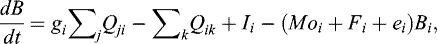 (1)
where gi is the dietary efficiency rate, Qji is the consumption of prey j by group i, Qik is the consumption of group i by predator k, Ii is immigration expressed in t/km2, Moi is the annual natural mortality other than predation, Fi is the annual fishing mortality rate and ei is the annual emigration rate. The predator–prey relationship that determines consumption Qji is based on foraging arena theory in which the biomass of prey is divided into a vulnerable compartment and a non-vulnerable compartment with respect to its predator (Walters and Kitchell, 2001; Ahrens et al., 2012). The transfer rate between these two compartments (called the vulnerability parameter) varies from 1 to infinity. In practice, the vulnerability is the maximum multiplier of the mortality rate that a predator can have on a prey. A high vulnerability value implies that a change in predator biomass causes variation in the biomass of its prey and thus the predator exerts a top-down control on its prey. In contrast, vulnerability equal to one indicates that the changes in prey biomass are independent of variation in predator biomass and thus are bottom-up controlled, depending on the environment. Theoretically, the vulnerability parameter can be estimated for each predator–prey pair during the fit of the model to time series. However, given the uncertainty of variation among the different prey of a given predator, and to reduce the number of parameters to estimate, it is common during the fitting phase of Ecosim models to assign identical values to all the prey for a given predator.
(1)
where gi is the dietary efficiency rate, Qji is the consumption of prey j by group i, Qik is the consumption of group i by predator k, Ii is immigration expressed in t/km2, Moi is the annual natural mortality other than predation, Fi is the annual fishing mortality rate and ei is the annual emigration rate. The predator–prey relationship that determines consumption Qji is based on foraging arena theory in which the biomass of prey is divided into a vulnerable compartment and a non-vulnerable compartment with respect to its predator (Walters and Kitchell, 2001; Ahrens et al., 2012). The transfer rate between these two compartments (called the vulnerability parameter) varies from 1 to infinity. In practice, the vulnerability is the maximum multiplier of the mortality rate that a predator can have on a prey. A high vulnerability value implies that a change in predator biomass causes variation in the biomass of its prey and thus the predator exerts a top-down control on its prey. In contrast, vulnerability equal to one indicates that the changes in prey biomass are independent of variation in predator biomass and thus are bottom-up controlled, depending on the environment. Theoretically, the vulnerability parameter can be estimated for each predator–prey pair during the fit of the model to time series. However, given the uncertainty of variation among the different prey of a given predator, and to reduce the number of parameters to estimate, it is common during the fitting phase of Ecosim models to assign identical values to all the prey for a given predator.
By using the 1980 Ecopath model as a starting point, the Ecosim model was fit to the time series data on fishery mortalities, biomass and catches for the 1980–2012 period. Fishing mortality in each of the ICES stock assessments was used as the forcing variable in the adjustment. Fishing mortality at age 1 was used for juvenile cod and hake, and the fishing mortality for haddock was assumed to be representative of the fishing pressure on the large demersal group. The biomass time series data are available in absolute values (in t/km2) for the 11 ICES-assessed groups and for juvenile cod and hake (biomass at age 1). The relative values of biomass indices were used for the large and medium demersal fish groups based on the estimation of biomass for haddock and boarfish, respectively, as well as for monkfish for which ICES provides biomass indices since 1997 based on scientific survey data. The time series of catches are available for the 29 groups of exploited species from ICES working group reports for assessed fish stocks and from the Statlant database for the other species.
We tried without success to improve the fit of the model using various environmental parameters (from Huret et al., 2013), particularly the sea–surface temperature and the North Atlantic oscillation index, as forcing functions. Following the procedure described by Christensen et al. (in press), we used recruitment anomalies as environmental variables to improve the Ecosim model fit, for groups whose dynamics are highly dependent on recruitment. Thus, the procedure was applied to juvenile hake, juvenile cod and small pelagic fish (anchovy, mackerel, horse mackerel and herring), assuming that the dynamics of these four stocks were similar to those of their recruits, given their short lifespan and high dependence on environmental conditions. For each group considered, anomalies were expressed as annual recruitment (estimated from ICES assessments) relative to mean recruitment for the study period. Then, they were used as forcing functions, thereby affecting the productivity of prey consumed by the group. We checked a posterior that the procedure improved the global fit of the model to the time series.
2.4 EcoTroph models
The EcoTroph model (Gascuel, 2005; Gascuel and Pauly, 2009) is based on a simple representation of the ecosystem using trophic spectra that represent the continuous distribution of the main ecosystem parameters as a function of trophic level τ (Gascuel et al., 2005). This continuous distribution is conventionally approximated by considering trophic classes of Δτ = 0.1 trophic level (TL) in width (i.e. Bτ designates the biomass of trophic class [τ, τ+Δτ]). Using the Ecopath model as a starting point, trophic spectra were constructed for biomass, production, total catch and respiration. To do this, the biomass Bi (or production Pi = Bi × (P/B)i, or catch Yi, or respiration Ri = Bi × (R/B)i) of each Ecopath functional group i is distributed across a range of trophic levels according to a log-normal distribution, to account for inter-individual variability within each group. The sum of the biomass (or production, or catches or respiration) of all groups constitutes the biomass (or production or catches or respiration) trophic spectrum (for the detailed procedure of spectrum construction, see Gasche et al., 2012; Colleter et al., 2013). From these, trophic spectra can be deduced for kinetics (Kτ = Pτ/Bτ), fishing mortalities (Fτ = Yτ/Bτ) and fishing loss rate (φτ = Yτ/Pτ). Trophic spectra were used to carry out a global comparison of the outputs of the 1980 and 2012 Ecopath models.
The EcoTroph model was then used to simulate changes in fishing pressure by modifying the fishing mortality parameter Fτ currently applied to each trophic class. The model is based on the assumption that ecosystem functioning can be represented as a simple continuous transfer of biomass from low to high trophic levels through predation and ontogeny (Gascuel, 2005; Gascuel and Pauly, 2009). This trophic flow is characterised by two parameters: biomass flow, which measures the quantity of biomass transferred to each trophic level per unit time (t km−2 yr−1), and the kinetics of that flow, which measures the velocity of the biomass transfers, i.e. the number of trophic levels τ crossed per unit time (TL yr−1). Based on these two parameters, the model can be constructed from four main equations derived from fluid mechanics.
The biomass equation links biomass Bτ (t km−2) to production Pτ (t TL km−2 yr−1), biomass flow Φτ and flow kinetics Kτ:
 (2)
(2)
The flow equation reflects that biomass transfers to higher trophic levels are not conservative. Losses occur due to, in part, the natural processes of respiration and excretion and, in part, to fishing. Thus:
 (3)
where μτ and φτ are the natural loss rate and the fishing loss rate, respectively. Exp(−μτ) is the trophic efficiency.
(3)
where μτ and φτ are the natural loss rate and the fishing loss rate, respectively. Exp(−μτ) is the trophic efficiency.
The kinetics equation (Gascuel et al., 2008) describes changes in life expectancy and thus the transfer velocity through the food chain caused by fishing and changes in predator abundance:
 (4)
where Kτ,bas, Fτ,bas and Bpred,bas designate the kinetics, fishing mortality and predator biomass (conventionally counted in the interval of [τ+0.8; τ+1.3]) respectively, in a baseline situation. Kτ and Bpred are the simulated velocity and biomass respectively, for a given value of fishing mortality Fτ. According to this equation, the speed of flow at trophic level τ depends partly on the abundance of predators Bpred. As a result, equation (4) introduces top-down control into the model. The coefficient α defines the intensity of this control and may vary between 0 (no top-down control) and 1 (all natural mortality Mτ depends on predator abundance). The coefficient γ is a shape parameter varying between 0 and 1, defining the functional relationship between predators and prey.
(4)
where Kτ,bas, Fτ,bas and Bpred,bas designate the kinetics, fishing mortality and predator biomass (conventionally counted in the interval of [τ+0.8; τ+1.3]) respectively, in a baseline situation. Kτ and Bpred are the simulated velocity and biomass respectively, for a given value of fishing mortality Fτ. According to this equation, the speed of flow at trophic level τ depends partly on the abundance of predators Bpred. As a result, equation (4) introduces top-down control into the model. The coefficient α defines the intensity of this control and may vary between 0 (no top-down control) and 1 (all natural mortality Mτ depends on predator abundance). The coefficient γ is a shape parameter varying between 0 and 1, defining the functional relationship between predators and prey.
The catch equation can be determined from the previous equations:
 (5)
(5)
Biomass and catch simulations were carried out using either the 1980 or the 2012 Ecopath models, to define the baseline situation required in equation (4). The corresponding trophic spectra define the values Bτ,bas, Pτ,bas, Fτ,bas and φτ,bas, from which are deduced the values of Kτ,bas (from Eq. (2)) and μτ,bas (from Eq. (3)). The latter parameter, as well as Φ1, the biomass flow at trophic level 1, were assumed independent of fishing and were thus valid for all simulations. Increases or decreases in fishing pressure were simulated considering a multiplier of fishing mortality mF varying between 0 (simulation of a no fishing scenario) and 3, with mF = 1 corresponding to the baseline situation. Thus for each simulation, the fishing mortality value Fτ = mF × Fτ,bas and the corresponding loss rate φτ = mF × φτ,bas were used to calculate the biomass flow Φτ (Eq. (3)), the flow velocity Kτ (Eq. (4)), and biomass Bτ of each trophic level (Eq. (2)). As kinetics and biomass are inter-dependent, equations (2) and (4) have to be solved using an iterative procedure, which starts with the baseline values Bτ,bas, then successively estimates Kτ and Bτ for each iteration, and continues until output values stabilise.
To make the model realistic, the most recent version of EcoTroph (Gascuel et al., 2011) distinguishes two compartments, one accessible to fishing and the other not, both characterised by different transfer velocities. This complexity is necessary because the kinetics of low or intermediate trophic levels are effectively very different between fished species (e.g. small pelagics or large crustaceans) and non-fished species (e.g. zooplankton). Equations (2)–(4) were thus applied, using distinct parameters, to the whole ecosystem on the one hand, and only to the fishing-accessible or fishable fraction (whose parameters are noted  , etc.) on the other hand. Parameters related to the fishable biomass were estimated for the baseline situation by determining, for each trophic box in the associated Ecopath model, a fishing accessibility coefficient that varies from 0 to 1 and by constructing the corresponding spectra. The accessibility of a group theoretically measures the proportion of biomass that would disappear in an infinite fishing effort (Gascuel et al., 2011). Thus, accessibility is generally less than 1 (see Table 2) due to: selectivity that protects juveniles, the refuge effect in areas inaccessible to fishing operations, the presence of non-fished species within certain Ecopath multispecific groups and the permanent arrival of fish via dispersal or migration for species whose distribution range is larger than the study area. The link between total biomass and the accessible fraction is expressed in the parameter
  , also calculated in the baseline situation. Thus, this parameter measures the resultant between natural losses that occur during trophic transfers and gains linked to the conversion of inaccessible biomass into accessible biomass (e.g. when fish eat zooplankton). Ultimately, catches are calculated by applying equation (5) to the fished fraction of the ecosystem.
The model was implemented in this study using the R-EcoTroph package developed by Colleter et al. (2013) and by using the default values for the parameters α and γ (0.4 and 0.5, respectively). The package includes two sub-routines: ET-Transpose, which builds all trophic spectra derived from the pre-existing Ecopath model, and ET-Diagnonis, which performs simulations of increasing or decreasing fishing mortalities, using the same fishing mortality multiplier for all trophic classes (mF from 0 to 3.0). Based on the same kind of simulations, the package also calculates two fishing indicators: mFMSY,τ is the fishing mortality multiplier that ensures a maximum sustainable yield for trophic class τ (thus overfishing occurs at level τ when mFMSY,τ < 1), and mF0.1,τ is the fishing mortality multiplier corresponding to the slope of the catches curve equal to 10% of the original slope (Gasche et al., 2012). The mF0.1,τ indicator is analogous to F0.1 typically used in stock assessments. By convention, the value mF0.1,τ = 1 defines the lower limit of the full exploitation. Therefore, the trophic class τ is underexploited when mF0.1,τ > 1, and fully exploited when mF0.1,τ ≤ 1 and mFMSY,τ ≥ 1.
2.5 Ecosystem indices
For a complementary diagnosis of the impact of fishing in the Celtic/Biscay system, four ecosystem indicators were calculated from the predicted annual biomass in the Ecosim model for the 1980–2012 period.
The mean trophic level (MTL) of the biomass in the ecosystem measures the impact of fishing on the entire trophic network (Jiming, 1982; Pauly et al., 1998). It is calculated as follows:
 (6)
where Bs is the total biomass of species s found in the studied ecosystem and TLs is its mean trophic level.
(6)
where Bs is the total biomass of species s found in the studied ecosystem and TLs is its mean trophic level.
The marine trophic index (MTI) reflects the changes in species composition among the predators in the ecosystem and thus measures the impact of fishing on high trophic levels (Pauly and Watson, 2005). It is defined as the mean trophic level of species having a trophic level greater than 3.25. Thus the calculation of MTI excludes planktivorous species whose variation in abundance depends mainly on environmental conditions.
The high trophic level indicator (HTI) is a new indicator proposed by Bourdaud et al. (2016) to measure the impact of fishing on high trophic levels. It quantifies the abundance of apex predators (TL > 4) within the total biomass of consumers (TL > 2) in the ecosystem.
 (7)
(7)
The apex predator indicator (API), also developed by Bourdaud et al. (2016), is defined in analogy to MTI. It quantifies the fraction of biomass attributed to apex predators (TL > 4) relative to the biomass of the ecosystem with a trophic level greater than 3.25.
 (8)
(8)
3 Results
3.1 Trend in biomass from surveys and catch
One of the main changes recorded in the Celtic/Biscay ecosystem was the succession of three dominant species of forage fish within 20 years: mackerel, followed by horse mackerel and then by boarfish (Fig. 2a). Mackerel biomass dropped from 1.2 Mt in 1980 to 0.15 Mt in 1985. During this same period, horse mackerel, which was then little exploited, had exceptionally high recruitment in 1982 leading to a strong increase in its biomass from 0.8 Mt to more than 2.8 Mt. This shift led to a change in fishing strategy with a considerable increase in fishing mortality for the horse mackerel, rising from 0.04 yr−1 in 1986 to 0.23 yr−1 in 1993. As a result, catches also increased rapidly and reached their highest values in 1997 (Fig. 2c), whereas its biomass dropped to 1.15 Mt. This decrease was concomitant to an increase in the abundance of boarfish, whose biomass doubled from 0.4 to 0.8 Mt between 1991 and 1998, which then grew further, exceeding 1 Mt since 2010. The boarfish has only a few potential predators and was not a fishing target until recently. However, boarfish landings have greatly increased in the past years, increasing from 35 t in 2001 to more than 80 000 t in 2012, while the biomass of the horse mackerel continued to decrease and was estimated at 0.53 Mt in 2012, a five-fold decrease compared with 1986.
The abundance of the other small pelagic fish (sardine, anchovy and herring) showed high variability likely due to environmental conditions, but also due to a pattern of marked increases, with cumulative biomass that went from approximately 0.5 Mt early in the study period to 1.5 Mt in the later years. Fishing mortality decreased in the mid-2000s, dropping from 0.16 yr−1 to less than 0.08 yr−1 on average (Fig. 2d), due mainly to a temporary increase in the biomass of horse mackerel and then the closing of the anchovy fishery between 2007 and 2009. In recent years fishing mortality was on the rise and reached its highest value in 2013 (0.26 yr−1), with fishing effort and catches increasing for boarfish, as well as for herring and horse mackerel.
Catches in the demersal group were remarkably stable between 150 000 and 200 000 t yr−1 over the study period. In contrast, biomass and fishing mortality showed pronounced changes over the last decade (Fig. 2b and d). Until the mid-2000s, mortality recorded in the ICES stock assessments fluctuated around a high mean value of the order of 0.5–0.6 yr−1 and biomass was low, ranging from 200 000 to 300 000 t. Between 2005 and 2010, fishing mortality was halved, whereas the total biomass of the seven fish stocks roughly doubled. This increase in biomass was mainly due to hake, and, to a lesser degree, to cod and whiting. Over the last two years of the study period, fishing effort appears to have increased (from 0.32 to 0.46 yr−1) although abundance was relatively stable.
 |
Fig. 2 Trends in stock biomass (a. for pelagics; b. for demersals), catches (c) and mean fishing mortalities (d), for species exploited in the Celtic/Biscay ecosystem. Catches refer to all species while biomass and fishing mortalities only include stocks assessed by ICES. For visual representation of trends, the missing biomass in the early period have been estimated proportionally to Statlant catches (hatched areas of time series; not used in the Ecosim model). |
3.2 Situation and trends of assessed stocks
The results of the ICES assessments confirmed the trends mentioned above. The mean B/Bpa ratio of the four demersal stocks (hake, haddock, cod and whiting) increased greatly during the end of the study period, rising from 1.1 in 2006 to 4.4 in 2011 (Fig. 3a). Fishing pressure was reduced by more than two-fold, going from a situation of high overfishing during the 1990s to a situation close to sustainable fishing in 2011 (F/FMSY ratio dropped from 2.40 to 0.98). However during the last years of the study period, fishing pressure was on the rise (F/FMSY = 1.1), whereas the mean biomass of the fish stocks significantly decreased (B/Bpa = 3.0). Moreover, the average ratio hides contrasts between demersal stocks. Among the four stocks studied here, only whiting and hake are currently found in the safe zone (Fig. 3c), a net improvement from 1980 (Fig. 3b). Although haddock have a biomass greater than the precautionary value Bpa, and higher than in 1980 (Fig. 3b), fishing mortality is still higher than the recommended FMSY value, while the biomass of cod is still severely depleted. The high biomass of hake and haddock was due to exceptional recruitment events during the latter years of the study period.
The average state of the ICES-assessed stocks of pelagic species showed three major periods. The first period from 1993 to 2001 was characterised by a degradation in the state of resources, with a decrease in the B/Bpa ratio from 1.94 to 0.83 and mean fishing mortalities similar to or greater than FMSY. By the early 2000s, the mean trajectory of pelagic resources was in the danger zone. The second period, from 2001 to 2009, was characterised by an overall improvement in the state of stocks. The F/FMSY ratio decreased from 1.05 to 0.5, whereas the relative abundance B/Bpa grew from 0.8 to 1.9. This increase more specifically involved herring and horse mackerel whose biomass increased three-fold during the period. In the third period covering the most recent years, fishing pressure increased, with 2015 showing a slight decrease in the mean biomass. However, the trajectory remains in the safe zone.
Although the last years of the study period appear to be characterised by inversion of the promising trends of the second period, there was an overall improvement in the state of fish resources studied between 1980 and 2015. Of the 11 ICES-assessed stocks, 8 were in the safe zone in 2015 (hake, plaice, mackerel, herring, whiting, sole VIIe and VIIfg, and horse mackerel; Fig. 3c), compared with three in 1980. On average, biomass increased, but remained below the Bpa precautionary limit in 2015 for 2 stocks (cod and sole 8ab), while the same sole 8ab and haddock were still overfished.
 |
Fig. 3 Diagnosis of stocks status for stocks assessed by ICES: (top) 1993/2015 mean trajectories of relative biomass (B/Bpa) and fishing mortalities (F/FMSY) for demersals (haddock, hake, cod and whiting) and pelagics (mackerel, horse mackerel and herring); (middle and bottom) stocks status in 1980 (or for the first year of assessment; see Table 1) and in 2015. |
3.3 Ecopath models: change in the ecosystem between 1980 and 2012
The 2012 Ecopath model of the Celtic/Biscay ecosystem accounts for a total biomass of 165 t km−2 (excluding detritus) and a biomass of animals (thus excluding primary producers) of 100 t km−2 (Table 2). With the exception of the small bathydemersal group, all the upper trophic levels in the ecosystem were exploited (Fig. 4). The highest tropic level groups are sharks, toothed whales, hake and monkfish. The model enables to estimate the mixed trophic impact indices (Ulanowicz and Puccia, 1990) that measure the positive or negative impact of each fishery on each group (Fig. 5). Through model construction, catches of each fish stock constitute a distinct fishery that thus impacts the related stock. The strongest impacts were observed on cod and monkfish, followed by mackerel, megrim, sole and plaice. The mixed fishery – which conventionally aggregates unassessed catches – impacts mainly the large sharks and large demersal fish groups. Positive impacts were observed for whales, which took advantage of the fishing-induced release of predation on their prey. Given the compensatory effects linked to this increase in prey abundance, fishing had little impact on most pelagic fish (sardine, sprat, large and medium pelagics) or on various small and medium demersals and blue whiting.
The comparison of the 1980 and 2012 Ecopath models using trophic spectra extends the finding of ICES stock assessment analyses to the whole ecosystem (Fig. 6). Overall, fishing mortality was reduced for all the exploited trophic classes in the ecosystem. For the high trophic levels (TL between 4.0 and 4.8), primarily represented by demersal and large pelagic fish, mortality was close to 0.2 yr−1 in 1980. This value appears to be low, but the fishing loss rate of the exploited fraction (φ⁎ = Y/P⁎, which measures the actual pressure exerted on each trophic class) was greater than 0.8 TL−1, which, in contrast, is very high (80% of the production of the accessible biomass is harvested each year). Between 1980 and 2012, fishing mortality and loss rates decreased by 20 and 25%, respectively, while biomass increased (+25%) and catches remained relatively constant. In other words, the decrease in fishing pressure was accompanied by a recovery of stocks, for roughly equivalent catches.
For the intermediate trophic classes (TL 3.4–3.9), which contain small pelagics and demersals that are little- or non-exploited (i.e. small and medium demersals and bathydemersal fish), mean fishing mortality was lower than 0.15 yr−1 in 1980. The fishing loss rates of the accessible fraction were nevertheless high, with values greater than 0.7 TL−1. There was a strong decrease in fishing pressure (−35 and −45% for F and φ∗, respectively), but biomass remained relatively constant over the study period. In other words, the decrease in fishing pressure was not accompanied by an overall recovery of stocks. Thus, catches also decreased by 35%. The stability in biomass masked the changes in species composition, with in particular a decrease in mackerel (TL 3.6) and an increase in boarfish (TL 3.3).
Finally, given the very high non-exploited biomass, the fishing mortality applied to the lower trophic levels (TL 2.1–2.6) was negligible. The fishing loss rates applied to the fished fraction increased during the study period, from 0.08 to 0.14 TL−1, due mainly to the development of shell fishing. Catches increased in the same proportion (+80%).
The changes that occurred between 1980 and 2012 also affected more global parameters of ecosystem functioning (Fig. 6, bottom). Trophic flow kinetics estimated from EcoTroph increased (+10%) for trophic levels higher than 3.4, even though the decrease in fishing pressure was expected to have the opposite effect. This change can be attributed to changes in species composition characterised by an increase in short-lived trophic groups that have high flow velocity. Organisms thus had shorter lifespans within their trophic class, thereby reducing the biomass of the class. This shift has a compensation effect and may explain, at least in part, the absence of biomass growth in the intermediate trophic levels. In other words, while the fishing pressure decreased, the ecosystem was not coming back to the ante state. Changes that have occurred in species assemblages lead to faster transfers, inducing lower abundances at intermediate trophic levels. Furthermore, based on Ecopath outputs, losses due to respiration increased for these trophic classes (+20%). This increase was also related to changes in species composition and suggests a decrease in the trophic efficiency of the ecosystem, with more losses in the trophic transfers and therefore reduced biomass flow reaching the higher trophic levels.
 |
Fig. 4 Trophic network in the Celtic/Biscay ecosystem from the 2012 Ecopath model (trophic levels are on the y-axis; circle sizes are proportional to the Log of the biomass of each group; exploited groups are in dark grey and colours refer diet coefficients). |
 |
Fig. 5 Mixed trophic impact (MTI) of each theoretical fishery (each identified by a colour) on the various Ecopath trophic groups (from the 2012 Ecopath model). |
 |
Fig. 6 Comparison of the two periods 1980 and 2012 based on trophic spectra derived from the two Ecopath models. Top: fishing mortalities (yr−1) and fishing loss rates of the accessible biomass (TL−1) per trophic class. Middle: biomass (t km−2) and catches (t km−2 yr−1) per trophic class. Bottom: kinetics (TL yr−1) and respiration rate per trophic class. |
3.4 EcoTroph diagnosis
The simulations conducted with the EcoTroph model quantified the effects of different multipliers of fishing effort on the biomass trophic spectrum (Fig. 7a). They showed that the trophic classes between TL 2.5 and 3.3 were generally insensitive to fishing. These trophic classes involve some small pelagic fish, but also groups such as benthos, shrimps and large zooplankton, which have high biomass and high turnover rates. These groups are little or non-fished and take advantage of the fishing-induced release from predation due to the removal of predators via fishing. The impact of fishing is more noticeable in the trophic classes between TL 3.3 and 4.1, including mackerel and horse mackerel, but also groups that are partially fished such as cephalopods and various demersals. Fishing had its maximum impact on trophic classes greater than TL 4.2 in which almost all species are fished and do not benefit from fishing-induced release from predation. Thus, compared with a no-fishing situation, the current biomass of fished species has been reduced by 1.3-fold for trophic classes TL 2.5 and 3.0, by 2-fold for TL 3.5 and 4.0, by more than 4-fold for TL 4.5 and by practically 6-fold for TL 4.8 (which includes large sharks and the largest individuals of the main demersal stocks) (Fig. 7b).
In terms of catches (Fig. 7c and d), the EcoTroph simulations indicated that the total production of the Celtic/Biscay ecosystem in 2012 could theoretically increase by 25% if fishing effort were to double. The analysis by trophic class, however, shows that this increase only involved trophic classes TL 2.5 and 3.0. However, the catches in classes TL 3.5 and 4.0 would remain at the same level and those of higher classes would decline.
The fishing indicators mF0.1 and mFMSY help to establish an overall ecosystem-scale diagnosis (Fig. 8) by indicating which trophic classes were fully exploited (mF0.1 < 1 fishing effort must be reduced to reach F0.1, the conventional lower boundary of full exploitation) or overfished (mFMSY < 1 fishing effort must be reduced to reach the maximum sustainable yield of the trophic class). Simulations show that in 1980, full exploitation was attained for trophic classes between TL 3.4 and 4.2, with overfishing for trophic classes greater than TL 4.2. In 2012, the diagnosis confirmed a clear improvement of the state of exploitation in the ecosystem. The trophic classes between TL 3.4 and 4.1 thus shifted from full exploitation to underfished. This change was mainly due to the decrease in fishing pressure during this period. It also reflects in part the increase in biomass of groups that were little fished such as boarfish, blue whiting and pouts, whereas fishing pressure remained high on horse mackerel and mackerel. We also observed an improvement for trophic classes TL 4.2–4.4 that shifted from overfishing in 1980 to sustainable fishing in 2012. This trophic interval includes a number of important fish stocks such as cod, whiting, megrim, juvenile hake, large pelagics, etc. However, the trophic levels greater than TL 4.5 remained overfished.
 |
Fig. 7 Outputs of EcoTroph simulations of increasing or decreasing fishing efforts or mortalities: (a) changes in the biomass trophic spectrum (t km−2 per trophic classes); (b) relative biomass of various trophic classes expressed as a function of the fishing effort multiplier (standardized to 1 for mE = 1); (c) total catches (t km−2 yr−1) for all groups, for all groups whose trophic level is higher than 2, and for all groups whose trophic level is higher than 3.5; (d) relative catch for various trophic classes expressed as a function of the fishing effort multiplier (standardized to 1 for mE = 1). |
 |
Fig. 8 Indicators of the status of the resource per trophic class: values of the fishing effort multiplier leading to a full exploitation (E_0.1) or to overexploitation (E_MSY) in 1980 (left) and 2012 (right). |
3.5 Ecosim fitting and ecosystem indicators
Overall, the Ecosim model fit the available time series well and reproduced the main changes observed involving biomass and landings in the various fished groups (see Supplementary Materials S6 and S7). In particular, biomass and catches simulated in 2012 by Ecosim were close to the initial values used in the 2012 Ecopath model. Regarding biomass, the model correctly predicted the upward or downward trends that occurred between 1980 and 2012, for 11 of the 13 biomass data series available (Fig. S7). It correctly captured the major changes observed within the period for species like whiting, cod, hake, sole or plaice, while recruitment forcing explained a large proportion of variability observed in mackerel and horse mackerel. However, the model fit was poorer for some small pelagics (anchovy, sardine), for which abundance is likely to be governed more by environmental conditions than by fishing or the trophic system described in the model.
The trophic-level based indicators, derived from the Ecosim model, highlight trends in the overall status of the food web, as a component of the ecosystem health (Fig. 9). The mean trophic level of the ecosystem biomass (MTL) decreased at the beginning of the studied period and then remained at low level. In contrast, other trophic-based ecosystem indicators increased slightly over the whole period, with the exception of a drop in 1985 due to an exceptional horse mackerel recruitment episode in 1982. This increase appeared to accelerate after 2005, suggesting an overall improvement in the state of the ecosystem. However, the change was slight for the marine trophic index (MTI, 3.68–3.73), while the improvement appeared to be more pronounced for the high trophic level index that measures the proportion of predators in the ecosystem (HTI, 4.0% to 4.9%) and for the apex predator indicator (API, 22% to 31%). This increase in trophic indicators was primarily due to the increase in biomass in species with trophic levels greater than 4, such as whiting, blue whiting, monkfish, large pelagics, etc. It was also accompanied by an increase in the trophic level of apex predators, such as sharks, whose trophic level increased slightly from 4.76 in 1980 to 4.82 in 2012.
 |
Fig. 9 Trends in the trophic indicators derived from the Ecosim model: mean trophic level (MTL in TL), marine trophic index (MTI in TL), high trophic level indicator (HTI in %) and apex predator indicator (API in %). |
4 Discussion
4.1 Limits and scope of the Ecopath model
The construction of Ecopath models is based on summarising data from the literature and harmonising all available data. For all of the assessed stocks, we used catch statistics and estimations of biomass published by ICES working groups. Although some uncertainties remain, such statistical data series provide the best information available, covering the entire ecosystem under study. However, in case of stocks with a broad species distribution, the biomass found in the study area was estimated from landings on a surface pro-rata basis. For the unassessed groups, biomass data were missing and were thus estimated by the model, using expert values between 0.8 and 0.95 for the ecotrophic efficiency EE. Then, we checked the reliability of such biomass estimates, especially through examination of the realism of the derived fishing mortalities. Based on our experience, we argue that such a procedure is more robust than using densities issued from scientific surveys and arbitrary values of catchabilities, to estimate biomass as input of an Ecopath model. Indeed, the order of magnitude is usually better known for fishing mortalities F and ecotrophic efficiencies EE than for catchabilities q. In such an approach, using the common procedure of pedigree to assess the whole model quality (Pauly et al., 2000; Christensen and Walters, 2004), would be inappropriate, due to its standard assumptions (quality scores high for biomass from surveys and very low for biomass estimated by the model, whatever the procedure is).
The reliability of estimates also depends on the quality of the data used as inputs, particularly on the P/B and Q/B ratios estimated from empirical equations and the diet matrix. This matrix was based on an extensive review of scientific studies, taking into account close or similar ecosystems, but for a time period stretching from 1980 to 2006. It is likely the weak point of our model, which should thus be considered as a first approach that provides an overall picture of the ecosystem state. This model should be improved upon in the future, in particular by including the sampling and analysis of stomach contents, a programme that has been recently initiated by IFREMER. As a related consequence, it would be of little interest to include complex sensitivity analyses here, before improving the diet matrix reliability or without taking into account the (unknown) uncertainty on diet coefficients (as, for instance, the Monte Carlo EwE procedure currently does).
Another future model improvement should be to reconsider the ecosystem boundaries. Here, we chose to combine the two areas, the Celtic Sea and the Bay of Biscay, into one ecosystem because they belong to the same Large Marine Ecosystem (LME 24), there are several overlapping stocks (megrim, hake, small pelagics), and the dataset was homogeneous, being compiled from the Evohe surveys covering the entire study area. Nevertheless, ecosystem approaches implemented by the CIEM (ICES Ecoregion Advice, 2014) or as part of the Marine Strategy Framework Directive (MSFD) now consider these two distinct ecoregions, based on biogeography, faunal composition and oceanographic characteristics (bathymetry, ocean circulations, stratification). Splitting the model to distinguish the two ecosystems is a required step currently in progress (Moullec et al., 2017).
4.2 Overfishing and ecosystem diagnosis
Stock assessments and trophic modelling are clearly complementary approaches for diagnosing the state of an ecosystem (Shephard et al., 2014; Gascuel et al., 2016). Here, we showed that the Celtic/Biscay ecosystem was heavily fished during the 1980–2000 period. Despite the introduction of a common fisheries policy in 1983 and the first regulatory measures implemented in the 1980s and 1990s (Holden and Garrod, 1996), fishing pressure has remained very high, especially for demersal species. In 1980, eight of the eleven stocks studied were overfished, of which five were in critical condition with a biomass lower than the precautionary threshold. The ensuing European regulations were notoriously insufficient with, in particular, legal sizes lower than the sizes at first maturity and fishing mortalities that reached two to six times natural mortality (Froese et al., 2008; Guénette and Gascuel, 2012). This situation also meant that the vast majority of fished trophic classes were fully or overexploited.
The implementation of the precautionary approach in the late 1990s (ICES, 1999) marked the beginning of a clear reduction in fishing pressure. This reduction continued in 2009 with the initiation of the transitory fisheries management scheme to bring stocks to the fishing rate supposed to produce the maximum sustainable yield by 2015. During the last studied years, the actual fishing pressure measured by the catch-to-production ratio has thus decreased by 25–45% for trophic levels greater than 3.0. Overall, the diagnosis shows that the state of health of the ecosystem clearly improved. The biomass of predators and the trophic indices increased, while overfishing was observed in only the highest trophic levels (4.4 compared with 4.2 in 1980). However, this improvement was partly due to some exceptional recruitment events, in particular for hake and haddock.
For the most recent years, the study depicts an ecosystem that remains heavily exploited, with fishing mortalities that appear to be on the rise again. In 2015, three of the eleven assessed stocks are still overfished and/or severely depleted, as are more generally trophic levels greater than 4.4 in the last EcoTroph diagnosis. The apparently favourable situation for trophic levels lower than 4.4 masks some contrasts revealed in CIEM stock assessments as well as Ecosim simulations. Thus, the EcoTroph model leads to an overall diagnosis of sustainable fishing because it combines within a single trophic class overfished stocks such as mackerel, horse mackerel, sole or plaice, with little fished groups and those with high biomass such as boarfish, blue whiting, pouts and various crustaceans. Finally, in an ecosystem perspective, mean fishing mortality of demersal species remained higher than the FMSY target and much higher than the threshold of F = 0.8 × M recommended by Walters and Martell (2004). In contrast, mean fishing mortality of pelagic stocks was close to the FMSY level in 2015 and very close or even slightly below the threshold of F = 0.6 × M recommended by Patterson (1992).
4.3 Changes in the trophic functioning of the ecosystem
One of the major changes that occurred during the study period was the gradual replacement of mackerel and horse mackerel by less exploited species in the ecosystem, such as boarfish, blue whiting and pouts. These species with higher productivity seem to have taken advantage of the environmental changes but also of higher availability of their trophic resources, related to the fishing-induced reduction in abundance of their competitors. Boarfish in particular is a short-lived species, very common in the Mediterranean region. Blanchard and Vandermeirsch (2005) noted its high colonising capacity and attributed its increase in biomass to the significant increase in bottom temperatures in the Bay of Biscay, particularly during its reproductive season. This increase in biomass occurred at a time of high trophic availability, with an increase in abundance of one of its main prey Calanus helglandicus (WGWIDE, 2014) and the decrease in abundance of mackerel and horse mackerel, which are Calanus predators and thus compete with boarfish.
These changes in species composition modified ecosystem functioning. In particular, there was an increase in the kinetics of trophic transfers (see Fig. 6), although the decrease in fishing mortalities and thus increase in mean lifespan should lead to the opposite situation. Overall, such faster trophic transfers across the food web tend to reduce biomass present within each of the trophic classes (Gascuel et al., 2008; Gascuel and Pauly, 2009). This is a general rule of the trophic dynamics: faster transfers imply lower residence times and thus less biomass within each trophic class. Here, the increase in flow kinetics explains, at least in part, the relatively constant biomass at intermediate trophic levels. The anticipated gains from more precautionary fishing seems to be somewhat countered by an increase in the velocity of trophic transfers.
The overfishing that occurred during the study period thus seems to have favoured trophic groups characterised by more rapid turnovers and matter transfers. Generally, these groups exhibit higher resilience to fishing (Gascuel and Pauly, 2009). However, at the same time, the results showed a nearly 20% increase in the respiration rates in the intermediate trophic levels, reflecting a decrease in transfer efficiency. In other words, due to changes that have occurred in species assemblages, the transfer of biomass in the trophic network occurred more rapidly, with shorter residence times within each trophic class, but less efficiently with more losses when moving from low to high trophic levels. This decrease in transfer efficiency may explain in part the weak increase in biomass observed in high trophic levels.
In our model, increases in respiration were linked to changes in species composition of intermediate trophic levels. In particular, the abundance of species characterised by low respiration rates, such as mackerel and horse mackerel, decreased between 1980 and 2012, while herring and boarfish characterised by higher respiration rates increased. Such results should be considered with care due to the high uncertainty affecting respiration rates estimates in most Ecopath models, including ours. Nevertheless, published values based on experimental studies tend to confirm this pattern, with higher respiration rates for herring than for horse mackerel (Johnstone et al., 1993; Wardle et al., 1996).
On the other hand, respiration is a metabolic process that is closely related to temperature (Pauly and Moreau, 1997) and temperature increased significantly in the Bay of Biscay and Celtic Sea during the study period (Garcia-Soto et al., 2002; Chust et al., 2011; Planque et al., 2003). This possible effect of temperature on the efficiency of transfer within the trophic network has been cited as one of the major consequences of climate change (Cheung et al., 2013). The effect was not considered in our approach, but could be included in the EcoTroph model by changing the natural loss rate parameter (μτ) over time. In such case, losses in trophic transfers due to respiration would increase, and the food web functioning would become even less efficient.
Overall, our results clearly highlight how human-induced changes in species assemblages may affect the global functioning of marine ecosystems, with potential impacts on the whole food web efficiency. Even if also observed in other ecosystems (e.g. Anh et al., 2015, in Vietnam), such effects remain poorly studied in trophic ecology. In the Celtic/Biscay ecosystem, some of the observed changes seem to be characteristic of a disturbed ecosystem, sensu Odum (1969), with an increased dominance of short-lived, highly productive species (Kay et al., 1989; Christensen, 1995) and with an increasing respiration rate per unit biomass (Fath et al., 2004). Thus, although the reduction in fishing pressure has improved the situation for certain fished stocks, the recent reduction has not been accompanied by a verifiable recovery of ecosystem structure and functioning. This type of pattern has been observed in most European ecosystems (Gascuel et al., 2016) and confirms that ecosystem changes, and in particular those induced by fishing, involve relatively slow dynamics, with recovery times that require decades (Jackson et al., 2001; McCauley et al., 2015).
5 Conclusion
The case study of the Celtic/Biscay ecosystem illustrates the usefulness of trophic models such as Ecopath, Ecosim and EcoTroph as tools to guide fisheries management. These models cannot replace single-species approaches to stock assessment, which remain necessary in particular to predict short-term changes, assess short term different fisheries management strategies and calculate fishing quotas. The trophic models are complementary because they provide three types of results. First, they can generalise the diagnostic of the impact of fishing to the whole ecosystem. In particular, the ET-Diagnosis routine of the EcoTroph model (available as an EwE plugin on http://www.ecopath.org, or as an R package on http://cran.r-project.org/) estimates the functions of production established according to trophic class rather than by stock, as well as indicators that can identify which classes are sustainably fished and which are overfished. Second, trophic models help to understand the ecosystem functioning and interpret unexpected changes. In the case of the Celtic/Biscay ecosystem, there were for example changes in species composition in forage fish, undoubtedly due to climate change and fishing impacts. Such changes reflect deteriorating trophic functioning of the ecosystem, with biomass transfers within the trophic network that appear to be more rapid and probably less efficient. These changes in functioning can explain, at least in part, why the biomass of the ecosystem did not increased substantially, or at levels lower than that anticipated by the decrease in fishing pressure.
Third, trophic models are useful for fisheries management because they can explore various scenarios and long term impacts of policies such as MSY (e.g. STECF, 2015a and b). In the Celtic/Biscay system, scenario building remains to be developed and will be the focus of an upcoming research project. On the medium term, one major issue is the identification and assessment of trade-offs between various management goals that are currently defined on a stock-by-stock basis, and that can be incompatible at an ecosystem level. MSY management that the European Union is striving to set up will require compromises between fish stocks and fisheries. More generally, different management scenarios need to be assessed with the goal of minimising the long-term impact on the ecosystem as a whole. Trophic modelling thus appears as a key step for defining strategic options for the medium term and for setting up a veritable ecosystem approach to fisheries management.
Supplementary Material
DOI: 10.1051/alr/2017006.s001
Supplementary file supplied by authors.
Access Supplementary MaterialAcknowledgements
We thank all the stock assessment scientists whose dedicated work made this research possible. We also thank anonymous reviewers whose suggestions strengthened the paper.
References
- Ahrens RNM, Walters CJ, Christensen V. 2012. Foraging arena theory. Fish Fish 13 (4): 41–59. [CrossRef] [Google Scholar]
- Allen KR. 1971. Relation between production and biomass. J Fish Res Board Can 28: 1573–1581. [CrossRef] [Google Scholar]
- Anh PV, Everaert G, Goethals P, Vinh CT, De Laender F. 2015. Production and food web efficiency decrease as fishing activity increases in a coastal ecosystem. Estuar Coast Shelf Sci 165: 226–236. [CrossRef] [Google Scholar]
- Araújo JN, Mackinson S, Ellis JR, Hart PJB. 2005. An Ecopath model of the western English Channel ecosystem with an exploration of its dynamic properties. Cefas Lowestoft (UK): Science Series Technical Report n° 125, 45p. [Google Scholar]
- Araújo JN, Mackinson S, Stanford RJ, Hart PJB. 2008. Exploring fisheries strategies for the western English Channel using an ecosystem model. Ecol Model 210: 465–477. [CrossRef] [Google Scholar]
- Blanchard F, Vandermeirsch F. 2005. Warming and exponential abundance increase of the subtropical fish Capros aper in the Bay of Biscay (1973–2002). C R Biol 328: 505–509. [CrossRef] [PubMed] [Google Scholar]
- Bourdaud P, Gascuel D, Bentorcha A, Brind'Amour A. 2016. Trophic indicators and ecosystem-based management targets: a modelling approach. Ecol Ind 61: 588–601. [CrossRef] [Google Scholar]
- Cardinale M, Dörner H, Abella A, et al. 2013. Rebuilding EU fish stocks and fisheries, a process under way? Mar Policy 39: 43–52. [CrossRef] [Google Scholar]
- Cheung WWL, Sarmiento SL, Dunne J, et al. 2013. Shrinking of fishes exacerbates impacts of global ocean changes on marine ecosystems. Nat Clim Change 3: 254–258. [CrossRef] [Google Scholar]
- Christensen V. 1995. Ecosystem maturity – towards quantification. Ecol Model 77: 3–32. [CrossRef] [Google Scholar]
- Christensen V. 2013. Ecological networks in fisheries: predicting the future? Fisheries 38 (2): 76–81. [CrossRef] [Google Scholar]
- Christensen V, Pauly D. 1992. ECOPATH II – a software for balancing steady-state ecosystem models and calculating network characteristics. Ecol Model 61: 169–185. [CrossRef] [Google Scholar]
- Christensen V, Walters CJ. 2004. Ecopath with Ecosim: methods, capabilities and limitations. Ecol Model 172: 109–139. [CrossRef] [Google Scholar]
- Christensen V, Walters CJ, Pauly D. 2005. Ecopath with Ecosim: a user's guide. Fisheries Centre, University of British Columbia, Vancouver, November 2005 edition, 154 p. (available online at www.ecopath.org). [Google Scholar]
- Christensen V, Walters CJ, Ahrens R, et al. 2009. Database-driven models of the world's Large Marine Ecosystems. Ecol Model 220: 1984–1996. [CrossRef] [Google Scholar]
- Christensen V, De la Puente S, Sueiro JC, Walters CJ, Tam J, Majiluf P. in press. Toward ecosystem based management of the Peruvian upwelling ecosystem: six decades of change. Ecol Model. [Google Scholar]
- Chust G, Borja A, Caballero A, et al. 2011. Climate change impacts on coastal and pelagic environments in the southeastern Bay of Biscay. Clim Res 48: 307–332. [CrossRef] [Google Scholar]
- Coll M, Akoglu E, Arreguın-Sanchez F, et al. 2015. Modelling dynamic ecosystems: venturing beyond boundaries with the Ecopath approach. Rev Fish Biol Fish 25: 413–424. [CrossRef] [Google Scholar]
- Colleter, M, Guitton, J, Gascuel, D. 2013. An Introduction to the EcoTrophR package: analyzing aquatic ecosystem trophic network. R J 5(1): 98–107. [Google Scholar]
- Colleter M, Valls A, Guitton J, Gascuel D, Pauly D, Christensen V. 2015. Global overview of the applications of the Ecopath with Ecosim modeling approach using the EcoBase models repository. Ecol Model 302: 42–53. [CrossRef] [Google Scholar]
- European Commission. 2002. Council Regulation (EC) No. 2371/2002 of the 31 December 2002 on the conservation and sustainable exploitation of fisheries resources under the Common Fisheries Policy. [Google Scholar]
- European Commission. 2008a. The role of the CFP in implementing an ecosystem approach to marine management. Communication from the Commission to the Council and the European Parliament. COM/2008/0187 final. [Google Scholar]
- European Commission. 2008b. Directive 2008/56/EC of the European Parliament and of the Council of 17 June 2008 establishing a framework for community action in the field of marine environmental policy (Marine Strategy Framework Directive. [Google Scholar]
- European Commission. 2013. Regulation 1380/2013 of the European parliament and of the council of 11 December 2013 on the Common Fisheries Policy. [Google Scholar]
- Fath BD, Jørgensen SE, Patten BC, Straškraba M. 2004. Ecosystem growth and development. Biosystems 77: 213–228. [CrossRef] [PubMed] [Google Scholar]
- Fernandes PG, Cook RM. 2013. Reversal of fish stock decline in the Northeast Atlantic. Curr Biol 23: 1432–1437. [CrossRef] [PubMed] [Google Scholar]
- Froese R, Stern-Pirlot A, Winker H, Gascuel D. 2008. Size matters: how single-species management can contribute to ecosystem-based fisheries management. Fish Res 92: 231–241. [CrossRef] [Google Scholar]
- Fulton EA, Link J, Kaplan IC, et al. 2011. Lessons in modelling and management of marine ecosystems: the Atlantis experience. Fish Fish 12: 171–188. [CrossRef] [Google Scholar]
- Garcia SM, De Leiva M. 2005. Evolution of the state of fish stocks in the Northeast Atlantic within a precautionary framework, 1970-2003: a synoptic evaluation. ICES J Mar Sci 62: 1603–1608. [CrossRef] [Google Scholar]
- Garcia SM, Zerbi A, Aliaume C, Do Chi, T, Lasserre G. 2003. The ecosystem approach to fisheries. Issues, terminology, principles, institutional foundations, implementation and outlook. FAO Fisheries Technical Paper No. 443. Rome: FAO. [Google Scholar]
- Garcia-Soto C, Pingree RD, Valdés L. 2002. Navidad development in the southern Bay of Biscay: climate change and swoddy structure from remote sensing and in situ measurements. J Geophys Res: Oceans 107: 28–31. [CrossRef] [Google Scholar]
- Gasche L, Gascuel D, Shannon L, Shin Y-J. 2012. Global assessment of the fishing impacts on the Southern Benguela ecosystem using an EcoTroph modelling approach. J Mar Syst 90 (1): 1–12. [CrossRef] [Google Scholar]
- Gascuel D. 2005. The trophic-level based model: a theoretical approach of fishing effects on marine ecosystems. Ecol Model 189: 315–332. [CrossRef] [Google Scholar]
- Gascuel D, Pauly D. 2009. EcoTroph: modelling marine ecosystem functioning and impact of fishing. Ecol Model 220: 2885–2898. [CrossRef] [Google Scholar]
- Gascuel D, Bozec Y-M, Chassot E, Colomb A, Laurans M. 2005. The trophic spectrum: theory and application as an ecosystem indicator. ICES J Mar Sci 62: 443–452. [CrossRef] [Google Scholar]
- Gascuel D, Morissette L, Palomares MLD, Christensen V. 2008. Trophic flow kinetics in marine ecosystems: toward a theoretical approach to ecosystem functioning. Ecol Model 217: 33–47. [CrossRef] [Google Scholar]
- Gascuel D, Guénette S, Pauly D. 2011. The trophic-level based ecosystem modelling approach: theoretical overview and practical uses. ICES J Mar Sci 68: 1403–1416. [CrossRef] [Google Scholar]
- Gascuel D, Coll M, Fox C, et al. 2016. Fishing impact and environmental status in European seas: a diagnosis from stock assessments and ecosystem indicators. Fish Fish 17: 31–55. [CrossRef] [Google Scholar]
- Guénette S, Gascuel D. 2012. Shifting baselines in European fisheries: the case of the Celtic Sea and Bay of Biscay. Ocean Coast Manage 70: 10–21. [CrossRef] [Google Scholar]
- Heymans JJ, Coll M, Link JS, et al. 2016. Best practice in Ecopath with Ecosim food_web models for ecosystem-based management. Ecol Model 331: 173–184. [CrossRef] [Google Scholar]
- Heymans JJ, Howell KL, Ayers M, et al. 2011. Do we have enough information to apply the ecosystem approach to management of deep-sea fisheries? An example from the West of Scotland. ICES J Mar Sci 68: 265–280. [CrossRef] [Google Scholar]
- Hoenig JM. 1983. Empirical use of longevity data to estimate mortality-rates. Fish Bull 81 (4): 898–903. [Google Scholar]
- Holden M, Garrod D. 1996. The Common Fisheries Policy: origin, evaluation and future. Oxford: Fishing News Books. 288 pp. [Google Scholar]
- Huret M, Sourisseau M, Petitgas P, Struski C, Léger F, Lazure P. 2013. A multi-decadal hindcast of a physical-biogeochemical model and derived oceanographic indices in the Bay of Biscay. J Mar Syst 109–110 (Suppl): S77– S94. [CrossRef] [Google Scholar]
- ICES. 1999. Report of the ICES Advisory Committee on Fisheries Management, 1998. ICES Cooperative Research Report, 229 pp. [Google Scholar]
- ICES. 2014. Report of the Report of the Working Group on Widely Distributed Stocks (WGWIDE), 26 August–1 September 2014, ICES Headquarters, Copenhagen, Denmark. ICES CM 2014/A COM: 15, 938 pp. [Google Scholar]
- Jackson JB, Kirby MX, Berger WH, et al. 2001. Historical overfishing and the recent collapse of coastal ecosystems. Science 293: 629–638. [CrossRef] [PubMed] [Google Scholar]
- Jennings SJ, Rice JC. 2011. Towards an ecosystem approach to fisheries in Europe: a perspective on current progress and future directions. Fish Fish 12: 125–137. [CrossRef] [Google Scholar]
- Jiming Y. 1982. A tentative analysis of the trophic levels of North Sea fish. Mar Ecol Progr Ser 7: 247–252. [CrossRef] [Google Scholar]
- Johnstone ADF, Wardle CS, Almatar SM. 1993. Routine respiration rates of Atlantic mackerel, Scomber scombrus L, and herring, Clupea harengus L, at low activity levels. J Fish Biol 42: 149–151. [CrossRef] [Google Scholar]
- Kay JJ, Graham LA, Ulanowicz RE. A detailed guide to network analysis. In: Wulff F, Field JG, Mann KH, eds. Network analysis in marine ecology. Berlin, Heidelberg: Springer, 1989, pp. 15–61. [Google Scholar]
- Lai S, Steenbeek J, Buszowski J. 2009. EwE6: interoperability usage, capabilities, technology, structure and beyond. Fish Centre Res Rep 17: 130–131. [Google Scholar]
- Lassalle G, Gascuel D, Le Loc'h F, et al. 2012. An ecosystem approach for the assessment of fisheries impacts on marine top-predators: the Bay of Biscay case study. ICES J Mar Sci 69: 925–938. [CrossRef] [Google Scholar]
- Lauria V. 2012. Impacts of climate change and fisheries on the Celtic Sea ecosystem. PhD thesis, Plymouth University, UK, 248p. [Google Scholar]
- Link JS. 2010. Adding rigor to ecological network models by evaluating a set of pre-balanced diagnostics: a plea for PREBAL. Ecol Model 221: 13–21. [Google Scholar]
- Link J. 2011. Ecosystem-based fisheries management: confronting tradeoffs. Cambridge: Cambridge University Press. [Google Scholar]
- Lynam C, Mackinson S. 2015. How will fisheries management measures contribute towards the attainment of good environmental status for the North Sea ecosystem? Global Ecol Conserv 4: 160–175. [CrossRef] [Google Scholar]
- Mackinson S. 2014. Combined analyses reveal environmentally driven changes in the North Sea ecosystem and raise questions regarding what makes an ecosystem model's performance credible? Can J Fish Aquat Sci 71: 31–46. [CrossRef] [Google Scholar]
- Mackinson S, Daskalov G. 2007. An ecosystem model of the North Sea to support an ecosystem approach to fisheries management: description and parameterisation. Sci Ser Tech Rep Cefas Lowestoft 142: 196 pp. [Google Scholar]
- McCauley DJ, Pinsky ML, Palumbi SR, et al. 2015. Marine defaunation: animal loss in the global ocean. Science 347 (6219): 247. [CrossRef] [Google Scholar]
- Moullec F, Gascuel D, Bentorcha K, Guénette S, Robert M. 2017. Trophic models: what do we learn about Celtic Sea and Bay of Biscay ecosystems? J Mar Syst [in press]. [Google Scholar]
- Odum EP. 1969. The strategy of ecosystem development. Science 164: 262–270. [CrossRef] [PubMed] [Google Scholar]
- Palomares MLD, Pauly D. 1998. Predicting food consumption of fish populations as functions of mortality, food type, morphometrics, temperature and salinity. Mar Freshw Res 49: 447–453. [CrossRef] [Google Scholar]
- Patterson K. 1992. Fisheries for small pelagic species: an empirical approach to management targets. Rev Fish Biol Fish 2: 321–338. [CrossRef] [Google Scholar]
- Pauly D. 1980. On the interrelationships between natural mortality, growth parameters, and mean environmental temperature in 175 fish stocks. J Cons 39: 175–192. [CrossRef] [Google Scholar]
- Pauly D, Moreau J. 1997. Méthode pour l'évaluation des ressources halieutiques. Toulouse: Cépaduès-Éditions, p. 288. [Google Scholar]
- Pauly D, Watson R. 2005. Background and interpretation of the ‘Marine Trophic Index’ as a measure of biodiversity. Philos Trans R Soc B: Biol Sci 360: 415–423. [CrossRef] [PubMed] [Google Scholar]
- Pauly D, Christensen V, Dalsgaard J, Froese R, Torres F. 1998. Fishing down marine food webs. Science 279: 860–863. [CrossRef] [PubMed] [Google Scholar]
- Pauly D, Christensen V, Walter C. 2000. Ecopath, Ecosim, and Ecospace as tools for evaluating ecosystem impact of fisheries. ICES J Mar Sci 57: 697–706. [CrossRef] [Google Scholar]
- Planque B, Beillois P, Jegou AM, Lazure P, Petitgas P, Puillat I. 2003. Large-scale hydroclimatic variability in the Bay of Biscay: the 1990s in the context of interdecadal changes. ICES Mar Sci Sympos 219: 61–70. [Google Scholar]
- Pikitch EK, Santora C, Babcock EA, et al. 2004. Ecology: ecosystem-based fishery management. Science 305: 346–347. [CrossRef] [PubMed] [Google Scholar]
- Polovina JJ. 1984. Model of a coral reef ecosystem I. The ECOPATH model and its application to French Frigate Shoals. Coral Reefs 3: 1–11. [CrossRef] [Google Scholar]
- Rice JC. 2011. Managing fisheries well: delivering the promise of an Ecosystem Approach. Fish Fish 12: 209–231. [CrossRef] [Google Scholar]
- Shephard S, Rindorf A, Dickey-Collas M, Hintzen NT, Farnsworth K, Reid DG. 2014. Assessing the state of pelagic fish communities within an ecosystem approach and the European Marine Strategy Framework Directive. ICES J Mar Sci: J Cons, fsu005. [Google Scholar]
- Scientific, Technical and Economic Committee for Fisheries (STECF). 2015a. Evaluation of management plans: evaluation of the multi-annual plan for the North Sea demersal stocks (STECF-15-04). Publications Office of the European Union, Luxembourg, EUR 27232 EN, JRC 95959, 152 pp. [Google Scholar]
- Scientific, Technical and Economic Committee for Fisheries (STECF). 2015b. Multiannual management plans SWW and NWW (STECF-15-08). Publications Office of the European Union, Luxembourg, EUR 27406 EN, JRC 96964, 82 pp. [Google Scholar]
- Tomczak MT, Müller-Karulis B, Järv L, et al. 2009. Analysis of trophic networks and carbon flows in south-eastern Baltic coastal ecosystems. Progr Oceanogr 81: 111–131. [CrossRef] [Google Scholar]
- Tomczak MT, Niiranen S, Hjerne O, Blenckner T. 2012. Ecosystem flow dynamics in the Baltic Proper-Using a multi-trophic dataset as a basis for food-web modelling. Ecol Model 230: 123–147. [CrossRef] [Google Scholar]
- Ulanowicz RE, Puccia CJ. 1990. Mixed trophic impacts in ecosystems. Coenoses 5 (1): 7–16. [Google Scholar]
- UN. 2012. The future that we want. Outcome of the United Nations Conference on Sustainable Development. Rio de Janeiro, Brazil: UN. [Google Scholar]
- Walters C, Kitchell JF. 2001. Cultivation/depensation effects on juvenile survival and recruitment: implications for the theory of fishing. Can J Fish Aquat Sci 58: 39–50. [CrossRef] [Google Scholar]
- Walters CJ, Martell SJD. 2004. Fisheries ecology and management. Princeton University Press. 428 pp. [Google Scholar]
- Walters C, Christensen V, Pauly D. 1997. Structuring dynamic models of exploited ecosystems from trophic mass-balance assessments. Rev Fish Biol Fish 7: 139–172. [CrossRef] [Google Scholar]
- Wardle CS, Soofiani NM, O'Neill FG, Glass CW, Johnstone ADF. 1996. Measurements of aerobic metabolism of a school of horse mackerel at different swimming speeds. J Fish Biol 49: 854–862. [CrossRef] [Google Scholar]
Cite this article as: Bentorcha A, Gascuel D, Guénette S. 2017. Using trophic models to assess the impact of fishing in the Bay of Biscay and the Celtic Sea. Aquat. Living Resour. 30: 7
All Tables
Parameters for the stocks assessed by ICES: stock name, name of the ICES working group in charge of the assessment, distribution area (ICES subdivisions), natural and current fishing mortalities (y−1), targets values for the fishing mortalities FMSY, current values B and threshold value Bpa for the stock spawning biomass (tons), first year of assessment. All parameters were issued from ICES reports. Note that values of FMSY and Bpa are not estimated by ICES for 4 stocks.
Parameters of the 2012 Ecopath model of the Celtic/Biscay ecosystem (values in bold were estimated by Ecopath). TL: trophic level (dimensionless); B: biomass (t km−2); P/B: production/biomass (yr−1); Q/B: consumption/biomass (yr−1); EE: ecotrophic efficiency (dimensionless); P/Q: production/consumption (dimensionless); Y: landings (t km−2 yr−1); Acces.: accessibility to fishing (dimensionless) (see Supplementary Material S4 for the 1980 model).
All Figures
|
Fig. 1 Map of the study area (delimited with a heavy line). The Celtic Sea and the Bay of Biscay. |
| In the text | |
|
Fig. 2 Trends in stock biomass (a. for pelagics; b. for demersals), catches (c) and mean fishing mortalities (d), for species exploited in the Celtic/Biscay ecosystem. Catches refer to all species while biomass and fishing mortalities only include stocks assessed by ICES. For visual representation of trends, the missing biomass in the early period have been estimated proportionally to Statlant catches (hatched areas of time series; not used in the Ecosim model). |
| In the text | |
|
Fig. 3 Diagnosis of stocks status for stocks assessed by ICES: (top) 1993/2015 mean trajectories of relative biomass (B/Bpa) and fishing mortalities (F/FMSY) for demersals (haddock, hake, cod and whiting) and pelagics (mackerel, horse mackerel and herring); (middle and bottom) stocks status in 1980 (or for the first year of assessment; see Table 1) and in 2015. |
| In the text | |
|
Fig. 4 Trophic network in the Celtic/Biscay ecosystem from the 2012 Ecopath model (trophic levels are on the y-axis; circle sizes are proportional to the Log of the biomass of each group; exploited groups are in dark grey and colours refer diet coefficients). |
| In the text | |
|
Fig. 5 Mixed trophic impact (MTI) of each theoretical fishery (each identified by a colour) on the various Ecopath trophic groups (from the 2012 Ecopath model). |
| In the text | |
|
Fig. 6 Comparison of the two periods 1980 and 2012 based on trophic spectra derived from the two Ecopath models. Top: fishing mortalities (yr−1) and fishing loss rates of the accessible biomass (TL−1) per trophic class. Middle: biomass (t km−2) and catches (t km−2 yr−1) per trophic class. Bottom: kinetics (TL yr−1) and respiration rate per trophic class. |
| In the text | |
|
Fig. 7 Outputs of EcoTroph simulations of increasing or decreasing fishing efforts or mortalities: (a) changes in the biomass trophic spectrum (t km−2 per trophic classes); (b) relative biomass of various trophic classes expressed as a function of the fishing effort multiplier (standardized to 1 for mE = 1); (c) total catches (t km−2 yr−1) for all groups, for all groups whose trophic level is higher than 2, and for all groups whose trophic level is higher than 3.5; (d) relative catch for various trophic classes expressed as a function of the fishing effort multiplier (standardized to 1 for mE = 1). |
| In the text | |
|
Fig. 8 Indicators of the status of the resource per trophic class: values of the fishing effort multiplier leading to a full exploitation (E_0.1) or to overexploitation (E_MSY) in 1980 (left) and 2012 (right). |
| In the text | |
|
Fig. 9 Trends in the trophic indicators derived from the Ecosim model: mean trophic level (MTL in TL), marine trophic index (MTI in TL), high trophic level indicator (HTI in %) and apex predator indicator (API in %). |
| In the text | |
Current usage metrics show cumulative count of Article Views (full-text article views including HTML views, PDF and ePub downloads, according to the available data) and Abstracts Views on Vision4Press platform.
Data correspond to usage on the plateform after 2015. The current usage metrics is available 48-96 hours after online publication and is updated daily on week days.
Initial download of the metrics may take a while.