| Issue |
Aquat. Living Resour.
Volume 34, 2021
|
|
|---|---|---|
| Article Number | 8 | |
| Number of page(s) | 9 | |
| DOI | https://doi.org/10.1051/alr/2021003 | |
| Published online | 09 April 2021 | |
Research Article
Using length data to derive biological reference points for kiddi shrimp Parapenaeopsis stylifera (Milne Edwards, 1837) from the south-eastern Arabian Sea, India
ICAR − Central Marine Fisheries Research Institute, Ernakulam North P.O., Kerala 682018, India
* Corresponding author: This email address is being protected from spambots. You need JavaScript enabled to view it.
Handling Editor: AE David Kaplan
Received:
26
August
2020
Accepted:
17
February
2021
Abstract
Parapenaeopsis stylifera, a major commercial penaeid shrimp fishery resource in the Indian Ocean, has lacked adequate information on life history parameters for nearly two decades. In this study, growth and mortality parameters of P. stylifera from the southwest coast of India were estimated using length data and used to derive biological reference points for the species. The asymptotic length for females was L∞ = 131 mm; k = 1.1 y−1 and for males L∞ = 117 mm; k = 1.25 y−1. Mortality parameter estimates were Z = 4.42, M = 1.24, F = 3.18 y−1 and exploitation rate E = 0.72 for females; Z = 5.76, M = 1.39, F = 4.37 y−1 and E = 0.76 for males. Thomson and Bell yield biomass, Beverton and Holt yield per recruit, and relative yield per recruit models were applied to predict the stock status and length cohort analysis for estimating the stock size. The Beverton and Holt analysis gave Emax = 0.69 in females and 0.75 for males, which is below the Ecurrent values obtained for the sexes. The Thomson and Bell analysis indicated that if Fcurrent at which the yield is 121 460 t in females and in males 128 064 t is further increased, rise in yield will be modest. B/B0 and SB/SB0 at Fcurrent were 24% and 18% for females and 21% and 16% for males, respectively. Target reference point F0.1 and F0.5 at different levels of age at capture tc (0.5, 0.6, 0.7 and 0.8 yrs) was estimated by Beverton and Holt yield per recruit model. The outcome from these models forms integral inputs for multispecies/multigear tropical fisheries management. Parapenaeopsis stylifera is one of the inshore penaeid shrimp identified by the Marine Stewardship Council for certification from the region and, moreover, biological reference points are a prerequisite to assessment and management of tropical multispecies fisheries for ecosystem-based fisheries management.
Key words: Arabian Sea / growth / Parapenaeopsis stylifera / reference points / size at first maturity / shrimp / size frequency
© EDP Sciences 2021
1 Introduction
Shrimps from India, as frozen products, contribute substantially to the international export market. Indian waters are habitat to a plethora of marine decapod crustaceans, with more than 70 species of penaeid shrimps recorded from the region (Radhakrishnan et al., 2012). Major commercial shrimp landings are composed of species belonging to the genera Metapenaeus, Parapenaeopsis and Penaeus. Parapenaeosis stylifera is a major fishery resource on the southwest coast of the Indian subcontinent. The European Union, Japan and southeast Asian countries are the major export markets for the resource. The species is distributed in the Indian Ocean from Kuwait and Pakistan to Bangladesh (Farfante and Kensley, 1997). Fishable quantity has been reported from Malaysia (Hall, 1962), Sri Lanka (De Bruin, 1965) and Pakistan (Ahmad, 1957). Introduction of trawlers by the erstwhile Indo-Norwegian project during the 1950's lead to an organised fishery for shrimps in Kerala, although prior to this period P. stylifera was a common species in the markets (Menon, 1953). The estimated annual production of P. stylifera during 1982–1987 varied from 10 344 t to 17 675 t with an annual average of 13 963 t (Suseelan, 1989). In the present study, the annual catches fluctuated between 5 269 t (2011) to 14 106 t (2019) (Figure given in Supplementary file). The resource is caught in single day trawlers (44%), voyaging daily (starting early morning and returning noon), and on multiday trips (55%) ranging from 3 to 4 days of voyage.
Since penaeid shrimps are short-lived resources with high fishery/ecosystem importance, they need more frequent assessments to understand their stock status and to keep the probability of overfishing at acceptable levels. There are two recent studies, one from the north-eastern Arabian Sea by Mohsin et al. (2017) who worked out the stock status of the species in Pakistan waters using surplus production models, and the other by Mohsen (2017) on the population dynamics from the north-west of Qeshm Island, Iran but it has been almost two decades (Suseelan and Rajan, 1989; Suseelan et al. 1989; Geeta and Nair, 1992; Alagaraja et al., 1986; Sarada, 2002, Dineshbabu, 2005) since any information on its life history parameters were published from Indian waters. Derivation of biological reference points (BRP) at regular intervals and ascertaining the stock status of the resource is also a prerequisite to assessment and management of tropical multispecies fisheries for ecosystem-based fisheries management (EBFM). This fishery resource from Kerala is also a candidate for the Marine Stewardship Council (MSC) certification. The main objectives of this study were i) to estimate growth and mortality parameters of P. stylifera from Kerala, south-west coast of India, and ii) to derive biological reference points, using multiple statistical methods, based on the length frequency data collected from January 2011 to December 2019, for the efficient management of the stock of P. stylifera along the south-west coast of India. Different stock assessment methods are used and it is recommended to use several of them (Lleonart, 2002) “if possible” as a fishery is a complex system.
2 Materials and methods
2.1 Study area and sampling
A total of 13 530 P. stylifera individuals (6954 females and 6576 males) were obtained by random sampling between January 2011 and December 2019 at fortnightly intervals for length frequency studies from single-day trawlers (3–4 h voyage) operating from Neendakara fisheries harbour (8°.93′7″N 76°.53′8″E) in Kerala, south-west coast of India (Fig. 1). Samples were transported to the laboratory on ice. Since the vessels targeting the species bring the entire catch to the landing centre, the samples used in the analysis can be considered representative of the population.
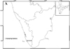 |
Fig. 1 Map showing study area. |
2.2 Data analysis
Shrimps were individually sexed, measured for total length from tip of the rostrum to the tip of the telson (to the nearest mm) and weighed in ‘g’, and size frequency distributions were constructed using size classes of 5 mm TL for 13 530 shrimps (51.39% females and 48.60% males) sampled. We measured the total length and weight only of those specimens with intact rostrum and telson. Specimens with broken rostrum/telson were discarded from the analysis. Given the biological differences between the sexes (growth and mortality rates), all the analyses were performed separately for males and females. Sex was determined by visual examination of the secondary sexual characters, namely thelycum in females and petasma in males. Length at age was established using von Bertalanffy growth equation (1938):
L∞, k and t0 were estimated from the length-frequency data using ELEFAN I with the FiSAT II program (FAO-ICLARM Fish Stock Assessment Tools, Version 1.2.2). L∞ is the asymptotic length, k is the von Bertalanffy growth constant and Lt is the expected length at age t years. t0 is the age at which the total length of the shrimp is zero and here in this study is considered zero as in most penaeid shrimps (Silva et al., 2019). Life span or the approximate maximum age tmax that a population would reach was calculated by the equation tmax = 3/k + t0 (Pauly and Munro, 1984).
Length/weight relationships were derived by applying the exponential equation: W = aLb, where W is the body weight (W, g), L is the length (L, cm), and ‘a’ and ‘b’ are constants. Size at 50% maturity in females was estimated using the King (1995) equation: P = 1/(1 + exp (−r(L − Lm)), where P is the predicted mature proportion, r = slope of the curve, and L = the total length. Proportion of sexually mature females were used in the analysis. Gonadosomatic index was determined using the equation: GSI = Weight of ovary/weight of shrimp × 100. Relative condition factor (Kn) was calculated as Kn = W0/Wc where W0 is the observed weight and Wc the calculated weight of shrimp, determined by inputting ‘a’ and ‘b’ values from the length/weight relationship (Le Cren, 1951).
Sex ratio was estimated each month and a Chi square (χ2) test (Snedecor and Cochran, 1967) on the sex ratio was performed, as is standard procedure to determine the significant variation in the frequency of each sex from the 1:1 ratio.
Total instantaneous mortality Z (Z, yr−1) was calculated from length converted catch curve analysis (Pauly, 1983), and natural mortality (M, yr−1) from Pauly's empirical formula (1980). Fishing mortality (F, yr−1) was calculated from the equation F = Z − M. The exploitation rate E was obtained from Gulland (1971): E = F/Z = F/(M + F).
Length cohort analysis (LCA) was used separately for the sexes to estimate the stock status, as LCA is used widely in tropical crustacean assessments (Sparre and Venema, 1998). Male Lm50 or length at which 50% of the individuals are mature was applied as 65 mm from Rao (1968) in LCA for males.
Thomson and Bell yield analysis (1934) was done to estimate the maximum sustainable yield (MSY), maximum economic yield, and the spawning stock biomass SSB, by inputting results obtained from LCA. The relative yield per recruit (Y'/R) and relative biomass per recruit (B'/R) of Beverton and Holt (1966), as modified by Pauly and Soriano (1986), was used to estimate the reference points − E0.1 (the exploitation level at which the marginal increase in yield per recruit reaches 1/10 of the marginal increase computed at a very low value of E), E0.5 (the exploitation level which will result in a reduction of the unexploited biomass by 50%) and Emax (the exploitation level that produces the maximum yield per recruit). Lc/Lα and M/K derived from ELEFAN I were used as input parameters. The yield per recruit (Y/R) at different age at capture (tc) by Beverton and Holt (1957) analysis was also conducted.
3 Results
3.1 Population structure, tmax, Lm and length at age
We collected 13 530 individuals of P. stylifera ranging in total length from 46 to 125 mm in females and 51 to 115 mm in males. In general, females were larger than males and dominated (p < 0.05) in the larger length classes (>80 mm TL). In the length classes up to 80 mm, males were dominant (Fig. 2). Length at age of females was 87 mm in the first year and 116 mm in the second year; 81 mm in the first year and 106 mm in the second year for males (Fig. 3).
Estimated size at 50% maturity was 71 mm TL in females (n = 580, R2 = 0.97). Minimum size at maturity (MSM) which is the smallest size at which the shrimps were mature was observed at 65–68 mm TL. Maximum life span was 2.7 in females and 2.3 in males.
 |
Fig. 2 Size frequency distribution of females and males of P. stylifera. |
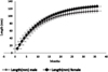 |
Fig. 3 Length at age for females and males of P. stylifera. |
3.2 Sex ratio, GSI and spawning period
Male to female ratio was 1:1.13. Chi square test (χ2) revealed dominance of females in the fishery during February (χ2 = 30.95, p < 0.05), March (χ2 = 5.45, p < 0.05), September (χ2 = 2.23, p < 0.05), October (χ2 = 7.42, p < 0.05) and November (χ2 = 3.57, p < 0.05), and in the remaining months followed 1:1 sex ratio. Spawning was continuous with peaks during April and September to December as maximum numbers of mature females were recorded during these months. Gonadosomatic index (GSI) revealed May (4.86) and December (4.49) as the peak spawning months in females (Fig. 4). Kn was observed to be above 1 during January to March, May, and August to December, with the highest value recorded in December for both females (1.18) and males (1.08).
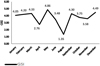 |
Fig. 4 Gonadosomatic index of P. stylifera females. |
3.3 Length/weight relationship
The length/weight regression was W = 0.00000118L3.3 (R2 = 0.77, n= 582) for females and W = 0.00000201L3.2 (R2 = 0.86, n = 580) for males. The difference between the slopes was not significantly different (p > 0.01) at 1%, hence the relationship for the pooled data was derived as W = 0.00000526L3 (R2 = 0.83, n = 1162) (Fig. 5).
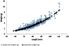 |
Fig. 5 Length/Weight relationship in pooled P. stylifera. |
3.4 Growth, mortality and recruitment
von Bertalanffy parameters L∞ and k obtained were 131 mm; K = 1.1 y−1 in females; 117 mm and 1.25 y−1 for males. Probability of capture was L25 = 67.58, L50 = 71.04 and L75 = 74.49 mm for females, and L25 = 64.57, L50 = 66.23 and L75 = 67.89 mm for males. Mortality parameters Z, M and F were 4.42, M = 1.24, F = 3.18 y−1 and E = 0.72 for females; Z = 5.76, M = 1.39, F = 4.37 y−1 and E = 0.76 for males (Figs. 6a and 6b). The data points on the initial ascending limb were excluded in the estimation of Z as these are length groups subject to lower fishing mortality because they are considered less vulnerable to the gear and thus might not have been fully recruited to the fishery or might have escaped the gear. The two length classes in females and one in males in the descending limb are comparatively less represented in the catch data. Hence these length groups were ignored.
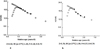 |
Fig. 6 Mortality in (a) female, and (b) male P. stylifera. |
3.5 Length cohort analysis
Length cohort analysis (LCA) was performed with inputs L∞, k, M and Lm50 values for females and males independently (Figure given in Supplementary file). Constants ‘a’ and ‘b’ values from the length/weight relationship were also included in the analysis. Highest fishing mortality was observed in the length range 101–105 mm TL in females and in males in the length range 86–90 mm.
3.6 Biological reference points
3.6.1 Thomson and Bell analysis
Results from LCA were input into the analysis. Figures 7a and 7b shows MSY, MSE and SSB of females and males, respectively at different F-factor. Yield at Fcurrent for females was 121 460 and males 128 064 t, which is close to the MSY level. Further increment in fishing pressure will not concede higher yield or financial returns. In contrast, a decrease in current fishing effort leads to maximum economic yield (MSE) at F = 0.8 and F = 0.6 in females and males, respectively. At these levels of fishing B/B0 and SSB/SSB0 are 27% and 22% in females, respectively and 30% and 25% in males, respectively. At Fcurrent, B/B0 and SB/SB0 are 24% and 18% for females, respectively and 21% and 16% for males, respectively.
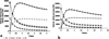 |
Fig. 7 Thomson and Bell analysis of yield/recruit for (a) female, and (b) male P. stylifera. |
3.6.2 Beverton and Holt yield per recruit analysis
F0.1 and F 0.5 were estimated from yield F curve at different age at capture tc (0.5, 0.6, 0.7 and 0.8 yrs) at current natural mortality M = 1.24 and 1.39 for females and males, respectively (Figs. 8a and 8b). F0.1is the fishing mortality where the slope of the yield per recruit curve is 10% of that at the origin and F0.5 is the fishing mortality that will reduce the equilibrium spawning potential per recruit to 50% to what it would be without fishing. Parameters used for the analysis were k = 1.1, W∞ = 11.8, t0 = 0, tr = 0.4, tc = {0.5, 0.6, 0.7, 0.8}, M = 1.24 for females, and k = 1.3, W∞ = 8.4, t0 = 0, tr = 0.4, tc = {0.5, 0.6, 0.7, 0.8} and M = 1.39 for males. Yield per recruit at Fcurrent ranged from 1.24–1.28 in females, and 1.33–1.43 in males. Fcurrent > F0.1 and F0.5 the conservative level of fishing for both the sexes.
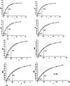 |
Fig. 8 Curves of yield per recruit on fishing mortality (F) for females (a) and males (b) estimated for age at capturet c = 0.5, 0.6, 0.7 and 0.8. |
3.6.3 Beverton and Holt relative yield per recruit (Y'/R) and relative biomass per recruit (B'/R)
Beverton and Holt relative yield per recruit analysis revealed Emax as 0.69, E50 = 0.37 and E10 = 0.60 for females and Emax = 0.75, E0.5 as 0.39 and E0.1 as 0.66 for males (Figs. 9a and 9b). The input parameters for the analysis, M/K ratio was 1 for both the sexes and Lc/L∞ = 0.53 for females and 0.59 for males, respectively. The reference points E0.1 is the level of exploitation at which the marginal increase in yield per recruit reaches 1/10 of the marginal increase computed at a very low value of E, E0.5 is the exploitation level which will result in exploitation of the unexploited biomass by 50% and Emax is the exploitation level that produces the maximum yield per recruit. Ecurrent for females and males (E = 0.72; E = 0.76) are higher than Emax, which indicates limiting exploitation rate to the conservative levels E0.1 or E50.
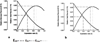 |
Fig. 9 Beverton and Holt yield/recruit for (a) female and (b) male P. stylifera. |
4 Discussion
The study estimated spawning period, length/weight relationship, growth, mortality and biological reference points leading to the stock status of P. stylifera using length data collected over a nine-year period at fortnightly intervals from trawler landings. The analysis is based on the data from single-day trawlers, mainly targeting the species and bringing the entire catch to the landing centre. Hence our data can be considered representative of the population of P. stylifera. Our observation on size range for the sexes were slightly more divergent than Suseelan (1989); Suseelan (1989) reported 35–100 mm size range for males and 35–115 mm for females. Again, in another study, Suseelan (1998) observed 46–100 mm in males and 46–125 in females, which is less than that reported in this paper. In penaeid shrimps, females generally reach larger sizes than males (Boschi, 1989), and the males have higher growth coefficients with lower asymptotic length, which is consistent with the findings in our study. Parapenaeopsis stylifera followed the reported trends of other tropical penaeid shrimps: faster growth, short life span completing its life cycle in 2.0–3 yrs (Garcia, 1988). Estimated Lm in this study is in accordance with Ramamurthy (1980), reported as 71 mm total length. Menon (1953) and Sarada (2002) recorded size at first maturity at 75 mm and 74.6 mmTL, respectively and Ayub (1998) from Pakistan observed size at maturity as 54 mm in males and 76 mm in females. Size at maturity is widely used as an indicator of minimum permissible capture size (Lucofora et al., 1999).
Previous investigations showed that the species spawn mainly in October-December in northern Kerala and in south Kerala during November, January and April (George et al., 1968; Rao, 1968). In Pakistani waters, spawning peak was during November to February (Ayub and Ahmed, 2002). Spawning periods may vary depending on the availability of food and other environmental fluctuations. Two spawning peaks were reported in other species of shrimps (Rao, 1968; Penn, 1980). In our study, two spawning peaks were also noticed (May and December) based on the highest values of the gonado-somatic index in females and during April and September to December, the percentage of mature females was at a maximum.
Length/weight relationship exhibited ‘b’ values as 3.2 and 3.3 for females and males, respectively and 3 for pooled data which agrees with the observation of Froese (2006) that the ‘b’ value in the length/weight relationship ranges between 2.5 and 3.5. The results of Kn, which were around one during most months, indicate a favourable environment for the growth of the species.
L∞ for the sexes concurred with previous studies on P. stylifera from Kerala (Suseelan, 1989; Sarada, 2002) (Tab. 1). The von Bertalanffy model (1938) is the most useful for the study of rapidly growing animals like penaeid and sergestid shrimps (Petriella and Boschi, 1997) as their growth is discontinuous. Z in our study was 4.42 for females and 5.76 for males. Most of the penaeid shrimp fisheries around the world have high fishing mortalities (Jones and Zalinge, 1981; Mehanna, 2000).
Yield per recruit models are very useful for single species approach to shrimp management and the models of Thomson and Bell and Beverton and Holt are widely used (Garcia, 1988) for stock assessment. Fishing at the MSY level does not necessarily maximise profits, but reduction of effort often leads to higher economic yield and higher spawning stock biomass. Reducing biomass to 25–30% of unexploited levels typically maximises their yields, while values beyond this level can result in losses of diversity and other ecological processes (McClanahan et al., 2011). Reducing present F to F0.1 or F0.5 which are target reference points would likely result in higher spawner biomass per recruit compared to current F. The conclusions of these Y/R models are very sensitive to seasonal patterns of recruitment, catchability, fishing effort etc. and more elaborate models are needed to fine tune management measures. This is especially the case when the problem of stock and recruitment relationship and uncertainty generated by non-fishery variables must be taken into account (Garcia, 1988). These models need to be applied in combination with stock recruit relationship (SRR) models to recognise the consequence of distinct management plans or strategies on egg production and yield. Understanding the relation between spawner abundance and subsequent recruitment is the most important issue in fisheries biology and management (Myers, 2007). Biological reference points, derived in this study by different models, can serve as an important supplement in fishery management plans. The BSM – Bayesian Schaefer Model, CMSY – Catch Maximum Sustainable Yield (Froese et al., 2017) are a step further in determining the stock status of the species. These methods can provide preliminary or prior reference points with reliable long time series of catch data, and also quantify the uncertainty of the parameter estimates. However, they do not consider the environment or stock interactions, factors for which models need to be developed. The best assessment is one that uses all the models that can be applied depending on available data and compares the results of all models, and the different results are used critically to gauge conclusions (Bonfil, 2005). In multi-species and multi-gear tropical fisheries, such inputs on major commercial resources form an integral part of holistic fishery assessments.
Comparison of growth parameters of P. stylifera between previous and present studies.
Supplementary Material
Supplementary file supplied by the authors. Access Supplementary Material
Acknowledgements
The authors thank the Director, ICAR-CMFRI for the facilities provided to carry out this work. A part of this work was presented during the 11th Indian Fisheries and Aquaculture Forum, Asian Fisheries Society, held during November 2017 inKochi, India.
References
- Ahmad N. 1957. Prawn and prawn fishery of East Pakistan. Directorate of Fisheries, Government of Pakistan, p. 43. [Google Scholar]
- Alagaraja K, George MJ, Narayana Kurup K, Suseelan C. 1986. Yield per recruit analysis on Parapenaopsis stylifera and Metapenaeus dobsoni from Kerala state, India. J Appl Ichthyol 2: 1–11. [Google Scholar]
- Ayub Z. 1998. A study of distribution, abundance and reproductive biology of Pakistani peaneaid shrimps, PhD thesis, University of Karachi, Karachi, Pakistan. [Google Scholar]
- Ayub Z, Ahmed M. 2002. Maturation and spawning of four commercially important penaeid shrimps of Pakistan. Indian J Mar Sci 31: 119–124. [Google Scholar]
- Bertalanffy LV. 1938. A quantitative theory of organic growth. Hum Biol 10: 181–213. [Google Scholar]
- Beverton RJH, Holt SJH. 1957. On the Dynamics of Exploited Fish Populations, Fish Invest Minist Agric Fish Food G G (2 Sea Fish), vol. 19, pp. 553. [Google Scholar]
- Beverton RJH, Holt SJH. 1966. Manual of methods for fish stock assessment. Part 2. Tables of yield functions. FAO Fish Technical Paper, vol. 38, pp. 67. [Google Scholar]
- Bonfil R. 2005. Fishery stock assessment models and their application to sharks, in: Management techniques for Elasmobranch fisheries, FAO Fisheries Technical Paper, Vol. 474, pp. 154–181. [Google Scholar]
- Boschi EE. 1989. Biología pesquera del langostino del litoral patagónico de Argentina (Pleoticus muelleri). Contribuciones INIDEP 646: 1–71. [Google Scholar]
- De Bruin GHP. 1965. Penaeid prawns of Ceylon (Crustacea Decapoda Penaeidae). Zool Meded Leiden 41: 73–104. [Google Scholar]
- Dineshbabu AP. 2005. Growth of Kiddi shrimp Parapenaeopsis stylifera (H. Milne Edwards, 1837) along Saurashtra coast. Indian J Fish 52: 165–170. [Google Scholar]
- Farfante IP, Kensley B. 1997. Penaeoid and Sergestoid shrimps and prawns of the world. Keys and diagnosis for the family and genera. Mus Natl Hist Nat 175: 232. [Google Scholar]
- Froese R. 2006. Cube law, condition factor and weight length relationships: history, meta-analysis and recommendations. J Appl Ichthyol 22: 241–253 [Google Scholar]
- Froese R, Demirel N, Coro G, Kleisner KM, Winker H. 2017. Estimating fisheries reference points from catch and resilience. (John Wiley and Sons Ltd). Fish Fish 18: 506–526. [Google Scholar]
- Garcia S. 1988. Tropical penaeid prawns, in: Fish Population Dynamics, 2nd edn, pp. 219–249. [Google Scholar]
- Geeta V, Balakrishnan Nair N. 1992. Reproductive biology of Parapenaeopsis stylifera . J Indian Fish Assoc 22: 1–12. [Google Scholar]
- George MJ, Raman K, Nair PK. 1968. Observations of the offshore prawn fishery of Cochin. Indian J Fish 10A: 460–499. [Google Scholar]
- Gulland JA. 1971. The Fish Resources of the Ocean, Fishing News (Books) West Byfleet. [Google Scholar]
- Hall DNF. 1962. Observations on the taxonomy and biology of some Indo West Pacific Penaeidae (Crustacea Decapoda). Fishery Publs. colon off 17: 229. [Google Scholar]
- Jones R, Van Zalinge NP. 1981. Estimates of mortality rates and population size for shrimp in Kuwait waters. Bull Mar Sci 9: 273–288. [Google Scholar]
- King M. 1995. Fisheries Biology, Assessment and Management, Fishing News Books, Oxford, p. 341. [Google Scholar]
- Le Cren ED. 1951. The length weight relationship and seasonal cycle in gonad weight and condition in the Perch (Perca fluviatilis). J Ani Ecol 20: 201–219. [Google Scholar]
- Lleonart J. 2002. Overview of stock assessment methods and their suitability to Mediterranean Fisheries, Fifth Session of the SAC-GFCM, Rome, pp. 37–49. [Google Scholar]
- Lucofora LO, Valero JL, Garcia VB. 1999. Length at maturity of the green eye spurdog shark Squalus mitsukuii (Elasmobranchii: Squalidae) from the SW Atlantic with comparisons with other regions. Mar Freshw Res 50: 629–632. [Google Scholar]
- McClanahan RT, Nicholas AJ, Graham M, Aaron MacNeil Nyawira A. Muthiga, Cinner JE, Bruggemann JH, Wilson SK. 2011. Critical thresholds and tangible targets for ecosystem based management of coral reef fisheries. PNAS 108: 17230–17233. [Google Scholar]
- Mehanna SF. 2000. Population dynamics of Penaeus semisulcatus in the Gulf of Suez, Egypt. Asian J Fish 13: 127–137. [Google Scholar]
- Menon MK. 1953. Notes on the bionomics and fishery of the prawn Parapenaeopsis stylifera (M. Edw) on the Malabar coast. J Zool Soc India 5: 153–162. [Google Scholar]
- Mohsin M, Mu Y, Memon AM, Kalharo MT, Shah SB, Hussain. 2017. Fishery stock assessment of Kiddi shrimp (Parapenaeopsis stylifera) in the Northern Arabian Sea Coast of Pakistan by using surplus production models. Chin J Oceanol Limnol 35: 936–946 . [Google Scholar]
- Mohsen S. 2017. Population dynamics of Kiddi shrimp Parapenaeopsis stylifera (H. Milne Edwards, 1837) in the north west of Qeshm Island, Iran. Tropical Zool 30: 13–27 . [Google Scholar]
- Myers AR. 2007. Stock and recruitment: generalizations about maximum reproductive rate, density dependence and variability using meta analytic approach. ICES J Mar Sci 58: 937–951 . [Google Scholar]
- Pauly D. 1980. On the interrelationships between natural mortality, growth parameters and mean environmental temperature in 175 fish stocks. J Cons CIEM 39: 175–192. [Google Scholar]
- Pauly D. 1983. Length converted catch curves: a powerful tool for fisheries research in the tropics (Part I): ICLARM Fishbyte 1: 9–13. [Google Scholar]
- Pauly D, Munro JL. 1984. Once more on growth comparison in fish and invertebrates. Fishbyte 2: 21. [Google Scholar]
- Pauly D, Soriano M. 1986. Some practical extensions to Beverton and Holts relative yield per recruit model, in: J.L. Mclean, L. Dizon, L. Hosillos (Eds.), The First Asian Fisheries Forum, Asian Fisheries Society, Manila, pp. 491– 495. [Google Scholar]
- Penn JW. 1980. Spawning and fecundity of the western King prawn Penaeus latisulcatus, Kishinouye, in Western Australian waters. Aust J Mar Freshw Res 31: 21–35. [Google Scholar]
- Petriella AM, Boschi EE. 1997. Growth of decapod crustaceans: Results of research made on Argentine species. Investig Mar 25: 135–157. [Google Scholar]
- Radhakrishnan EV, Deshmukh V.D, Maheswarudu G, Josileen Jose, Dineshbabu AP, Philippose KK, Sarada PT, Lakshmi Pillai S, Saleela KN, Chakraborthy Rekha D, Gyanranjan Dash, Sajeev CK, Thirumilu P, Sreedhara B, Muniyappa Y, Sawant AD, Vaidya NG, Johny Dias R, Verma JB, Baby PK, Unnikrishnan C, Ramachandran NP, Vairamani A, Palanichamy A, Radhakrishnan M, Raju B. 2012. Prawn fauna (Crustacea:Decapoda) of India: An annotated checklist of the penaeoid, sergestoid, stenopodid and caridean prawns. J Mar Biol Assoc India 54: 50–72. [Google Scholar]
- Ramamurthy S. 1980. Resource characteristics of the penaeid prawn Parapenaeopsis stylifera (Milne Edwards) in the Mangalore coast. Indian J Fish 27: 161–171. [Google Scholar]
- Rao PV. 1968. Maturation and spawning of the penaeid prawns of the southwest coast of India. FAO Fish Report 57: 285–304. [Google Scholar]
- Sarada PT. 2002. Fishery, biology and population dynamics of Parapenaeopsis stylifera at Calicut. Indian J Fish 49: 351–360. [Google Scholar]
- Silva EF, Calazans, N, Nole L, Soares R, Fredou LF, Peixoto S. 2019. Population dynamics of the white shrimp Litopenaeus Schmitti (Burkenroad, 1936) on the southeastern coast of Pernambuco, northeastern Brazil. J Mar Biol Assoc UK 99: 1–7 [Google Scholar]
- Snedecor GW, Cochran WC. 1967. Statistical Methods, 6th edn, Oxford and IBH Publishing Co., New Delhi, India, p. 593. [Google Scholar]
- Sparre P, Venema SC. 1998. Introduction to tropical fish stock assessment. FAO FisheriesTechnical Paper, 306/1. [Google Scholar]
- Suseelan C, Rajan KN, Nandakumar G. 1989. The Karikkadi fishery of Kerala. Mar Fish Infor Serv T E Ser 102: 4–8. [Google Scholar]
- Suseelan C, Rajan KN. 1989. Stock assessment of the kiddi shrimp Parapenaeopsis stylifera off Cochin, India, in: S.C. Venema, N.P. van Zalinge (Eds.), Contributions to tropical fish stock assessment in India, FAO/DANIDA/ICAR National follow up training course on fish stock assessment pp. 15–30. [Google Scholar]
- Thomson WF, Bell FH. 1934. Biological statistics of the Pacific halibut fishery 2. Effect of changes in intensity upon total yield per unit of gear. Rep Int Fish (Pacific Halibut) Comm 8: 49. [Google Scholar]
Cite this article as: Lakshmi Pillai S, Maheswarudu G, Baby PK, Radhakrishnan M, Ragesh N, Sreesanth L. 2021. Using length data to derive biological reference points for kiddi shrimp Parapenaeopsis stylifera (Milne Edwards, 1837) from the southeastern Arabian Sea, India. Aquat. Living Resour. 34: 8
All Tables
Comparison of growth parameters of P. stylifera between previous and present studies.
All Figures
|
Fig. 1 Map showing study area. |
| In the text | |
|
Fig. 2 Size frequency distribution of females and males of P. stylifera. |
| In the text | |
|
Fig. 3 Length at age for females and males of P. stylifera. |
| In the text | |
|
Fig. 4 Gonadosomatic index of P. stylifera females. |
| In the text | |
|
Fig. 5 Length/Weight relationship in pooled P. stylifera. |
| In the text | |
|
Fig. 6 Mortality in (a) female, and (b) male P. stylifera. |
| In the text | |
|
Fig. 7 Thomson and Bell analysis of yield/recruit for (a) female, and (b) male P. stylifera. |
| In the text | |
|
Fig. 8 Curves of yield per recruit on fishing mortality (F) for females (a) and males (b) estimated for age at capturet c = 0.5, 0.6, 0.7 and 0.8. |
| In the text | |
|
Fig. 9 Beverton and Holt yield/recruit for (a) female and (b) male P. stylifera. |
| In the text | |
Current usage metrics show cumulative count of Article Views (full-text article views including HTML views, PDF and ePub downloads, according to the available data) and Abstracts Views on Vision4Press platform.
Data correspond to usage on the plateform after 2015. The current usage metrics is available 48-96 hours after online publication and is updated daily on week days.
Initial download of the metrics may take a while.