| Issue |
Aquat. Living Resour.
Volume 33, 2020
|
|
|---|---|---|
| Article Number | 17 | |
| Number of page(s) | 11 | |
| DOI | https://doi.org/10.1051/alr/2020019 | |
| Published online | 16 November 2020 | |
Research Article
Model selection for fish growth patterns based on a Bayesian approach: A case study of five freshwater fish species
1
Department of Mathematics, Shandong University, Jinan 250100, PR China
2
South China Sea Fisheries Research Institute, Chinese Academy of Fishery Sciences, Guangzhou 510300, PR China
3
Key Laboratory of Open-Sea Fishery Development, Ministry of Agriculture and Rural Affairs, Guangzhou 510300, PR China
* Corresponding author: This email address is being protected from spambots. You need JavaScript enabled to view it.
Handling Editor: Verena Trenkel
Received:
3
May
2020
Accepted:
23
October
2020
Abstract
Selecting an appropriate growth pattern for individual fish is a meaningful but complex topic in fishery research. We model four growth functions − the commonly used von Bertalanffy growth model (VBGM), and the Gompertz growth model (GGM), Schnute–Richards growth model (SRGM), and generalized VBGM (G-VBGM) − to examine possible growth patterns. Mean total length-at-age fish datasets for five commercial fish species (yellow perch Perca flavescens, walleye Sander vitreus, northern pike Esox lucius, largemouth bass Micropterus salmoides and lake herring Coregonus artedi) from North American freshwater ecosystems, were analyzed. Using a Markov chain Monte Carlo (MCMC) algorithm, we structured four models combining informative priors of model parameters. It is the first time that deviance information criterion (DIC) and leave-one-out cross-validation (LOOCV) were combined to select the best growth model. During the model-selection process, the smooth LOOCV error successfully followed the trend of the LOOCV error, although there were difference in the curve shapes. Values of scale reduction factor (SRF) for all four models indicated convergence, ranging 1.02–1.06, below the 1.2 threshold. The GGM was selected for C. artedi, and the G-VBGM for the other four species. Our approach provided a robust process in model-selection uncertainty analysis, with the G-VBGM having the best prediction ability among our datasets.
Key words: Bayesian analysis / Fish growth models / Deviance information criterion / Markov Chain Monte Carlo / Leave-one-out cross-validation
© EDP Sciences 2020
1 Introduction
Deciding which fish individual growth model to use, or how to use it, can be difficult (Quinn and Deriso, 1999; Jonsson and Jonsson, 2009; Jessop, 2010), because many different types of models and approaches having been proposed to describe growth patterns (Cailliet et al., 2006; Haddon, 2010). Common practice among fishery scientists studying fish growth is to a priori adopt the most widely used function, the von Bertalanffy growth model (VBGM) (Kimura, 1980; Pilling et al., 2002; Chen et al., 2003; Cailliet et al., 2006; Katsanevakis and Maravelias, 2008).
The VBGM provides an empirical description of growth, and its usefulness for intra- and inter-population comparisons is widely recognized (Misra, 1986; Quinn and Deriso, 1999; He et al., 2005; Wilberg and Bence, 2008; Román-Román et al., 2010; Vilizzi and Copp, 2017). For example, Haddon et al. (2008) reported the VBGM had been used in 42 (71%) of abalone studies and the Gompertz growth model (GGM) (Gompertz, 1825) in only 4 studies (6.78%). However, the VBGM is not always the most appropriate function to represent the growth of a species (Katsanevakis, 2006; Haddon, 2010). For example, the generalized von Bertalanffy growth model (G-VBGM) has been developed for periods when the growth of individual fish differs, modeling length and weight in both isometric and allometric situations. (Szalai et al., 2003; Haddon, 2010; Román-Román et al., 2010).
Freshwater fishes face an array of threats, such as river fragmentation, dam construction, overexploitation, adverse species interactions, and pollution (Brosse et al., 2013; Kang et al., 2014). Accurate estimates of growth parameters are important for monitoring fish population status, as well as for assessing fisheries management decisions against external pressures (Zhu et al., 2016). We selected five freshwater fish species (northern pike Esox lucius and walleye Sander vitreus from Wabatongushi Lake (Northern Ontario), and yellow perch Perca flavescens, lake herring Coregonus artedi, and largemouth bass Micropterus salmoides from Lake Michigan) as model species for comparing alternative model formulations. These species support important fisheries (commercial and recreational), and are important components of food webs in the Great Lakes (Heyer et al., 2001; Eastwood and Couture, 2002; Helser and Lai, 2004; Jiao et al., 2006; Stockwell et al., 2006; Liu et al., 2017). In addition to VBGM, three other growth functions (Schnute-Richards growth model (SRGM), GGM, and G-VBGM) were included to model alternative growth patterns for these five fish species.
We used the Bayesian method to estimate model parameters (Michielsens and McAllister, 2004; Jiao et al., 2008; Wilberg and Bence, 2008; Brosse et al., 2013). Model performance was assessed by comparing goodness-of-fits and retrospective error evaluations (Michielsens and McAllister, 2004; Jiao et al., 2008; Nylander et al., 2008; Brosse et al., 2013). The Bayesian approach is widely regarded as the most important recent development in statistical computing, because it enables statisticians to essentially fit any probability model (Jiao et al., 2006; O'Hara and Sillanpää, 2009; Haddon, 2010). The deviance information criterion (DIC) of Spiegelhalter et al. (2002) enables comparison of a set of Bayesian models; it is similar to Akaike's information criterion (AIC), in combining a measure of goodness and complexity, and both are based on deviance. However, DIC provides an objective index, especially in models which differ in random effects or hierarchical structure, and is useful in situations where models are quite similar (Wilberg and Bence, 2008). Accordingly, DIC is widely used in a Bayesian framework for model selection; the smaller the DIC value the better a model fits the data (Spiegelhalter et al., 2002; Jiao et al., 2008; Wilberg and Bence, 2008).
Our aims were to (i) compare commonly used growth functions using Bayesian methods; (ii) recommend alternative fish growth models beyond those that are commonly used; and (iii) provide a best fitting growth model for five examined commercial fish species in North American freshwater ecosystems.
2 Materials and methods
2.1 Fish datasets
Fish length-at-age data for P. flavescens, C. artedi, E. lucius, S. vitreus, and M. salmoides were taken from Schneider (2000). Fishes were captured using multiple gears, such as gill nets, trap nets, seines, or by angling. Of these five species, E. lucius and S. vitreus were caught in Wabatongushi Lake, while P. flavescens, M. salmoides, and C. artedi were caught in Lake Michigan. While all species were sampled around the year, only individuals sampled in Jan–May were used. Individual fish age was determined by counting complete annuli (year marks) on scales; all fish considered to have a birthday on January 1. Therefore, fish collected between January 1 and the time an annulus was formed are regarded to be 1 year older than the number of annuli visible on a scale (Schneider, 2000). The back-calculation technique was also used for data collection. A linear relationship between fish total length and scale radius was fitted to calculate the average total length for each age (Schneider, 2000). The data used in this study consisted of mean total lengths (cm) at age (Tab. 1).
Mean total length (cm) and standard deviations (in brackets) by age group and number of observations for five freshwater fish species.
2.2 Growth models
Four growth models (VBGM, G-VBGM, GGM, SRGM) were assessed. VBGM is characterized by a concave length-at-age growth curve, while sigmoid curves, like GGM, portray growth traits with explicit inflection points (Katsanevakis and Maravelias, 2008). We focus on the development of fitting routines for highly flexible models, such as SRGM and G-VBGM. Information for all growth models is presented in Table 2.
Functions of the four growth models (VBGM, GGM, SRGM, G-VBGM) used in this study.
2.3 Model fitting
Lognormal distributions have been often used as informative priors in Bayesian analyses (Zellner, 1971). For growth models, growth coefficient k and asymptotic length L∞ have also been given lognormal prior distributions (Zhu et al., 2016). Following Zhu et al. (2016), we assumed informative lognormal prior distributions, with means µL, µk, and precisions (1/variance) τL, τk: (1)
(1)
 (2)
(2)
For other parameters relatively uninformative uniform priors were assumed (Tab. 3). The models were fitted using the Markov chain Monte Carlo (MCMC) algorithm. A normal likelihood for mean length-at-age was assumed for all four models: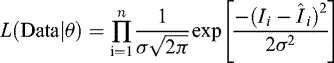 (3)where L(Data|θ) is the likelihood of the data given the parameter vector θ; θ denotes (L∞, k, t0, σ2), Ii and
  are values of observed and predicted mean length-at-age, respectively.
Mean and standard deviations (SD) for lognormal prior distributions used for asymptotic length (L∞) for five freshwater fish used in Bayesian analysis.
2.4 Model evaluation
The DIC was used to evaluate the relative goodness-of-fit of each growth model; the smaller the DIC value the better a model fits the data (Spiegelhalter et al., 2002; Jiao et al., 2008; Wilberg and Bence, 2008). The pD is a measure of the effective number of parameters in a model. It is calculated as the difference between the posterior mean of the deviance ( ) and the deviance at the posterior means of the parameters of interest (
 ) (Spiegelhalter et al., 2002):
 (4)
(4)
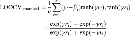
Leave-one-out cross-validation (LOOCV) is generally used to investigate model fit while preventing over-fitting of small datasets. Three LOOCV equations including LOOCV, smoothed LOOCV, and Bayesian LOOCV were used in this study. These LOOCV approaches can be computed with a small additional cost after obtaining the posterior approximation given the whole data. The LOOCV, smoothed LOOCV, Bayesian LOOCV, expected log-predictive density for a new mean length-at-age data point (elpdDIC), and the log pointwise predictive densities (lppdLOOCV), are defined as follows (Langaas et al., 2005; Bo et al., 2006; Gelman et al., 2014):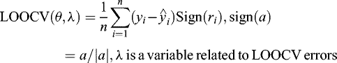 (5)
(5)
 (6)
(6)
 (7)
(7)
 (8)
(8)
 (9)where in equation (5), θ are model parameters, λ is a variate related to LOOCV errors (detailed computing process is shown in Bo et al., 2006), n is the number of estimates, the sign(a) is a function which equals to 1 if a ≥ 0 and −1 otherwise, yi and
  are the observed and estimated mean length-at age values for the ith data point, ri is the difference between the observed and estimated mean length-at age value for the ith data point. In equation (6), we set γ to be 10 (generally, it is difficult to select the optimal value of γ), the tanh(γri) is one of the hyperbolic functions. In equation (7), ppost(yi) denotes the posterior probability density of θ for yi and
  is the predicted density for
  . In equation (8), f denotes the data probability distribution. More details of LOOCV method can be found in Bo et al. (2006).
Convergence diagnostic analysis is important for judging the reliability of model results (Gelman and Rubin, 1992; Brooks and Roberts, 1998). A scale reduction factor (SRF) SRF >1.2 or SRF <1.0 indicates that parameters may not have converged for that chain. The mean intra-chain (W) and inter-chain (B) variances, and the SRF were calculated as follows: (10)
(10)
 (11)
(11)
 (12)where J is the number of MCMC chains, j is the serial numbers of the chains, G is the length of a chain, g is the serial numbers of estimated values, θgj is the gth estimated value in the jth chain of parameter θ, θj is the mean value of θ in the entire j sequence.
All analyses in this study were conducted using R (version 3.6.3) packages MASS, mvtnorm, R2jags, and CODA.
3 Results
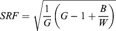
Posterior 95% credible interval estimates and posterior means of growth parameters (L∞, k, t0, r, g, p, v, δ, γ) were calculated for each growth model for each fish species (Tab. 4). The VBGM led to a smaller L∞ estimates and larger k estimates than the generalized form (G-VBGM) for E. lucius, S. vitreus, P. flavescens, and C. artedi. Posterior parameter estimates were largely influenced by the rather informative prior distributions (e.g. G-VBGM in Fig. 1). Of the four models, G-VBGM always produced the largest L∞ posterior estimates, except for M. salmoides. The smallest L∞ estimates were generated by the GGM for P. flavescens, S. vitreus, and M. salmoides, by the SRGM for C. artedi, and the VBGM for E. lucius (Tab. 4).
The G-VBGM was the best fitting model with the lowest DIC values for P. flavescens (259.51), S. vitreus (263.37), E. lucius (260.84), and M. salmoides (261.35) while the GGM had the lowest DIC (250.62) for C. artedi (Tab. 5).
Convergence diagnostics (using SRF) for the four models determined if a model produced reliable results. An SRF <1.2 indicates good mixing and convergence of MCMC chains, within the total number of MCMC iterations (<30,000). The SRF values for the parameters of all four models indicated convergence, ranging 1.02–1.06.
For all species except C. artedi the G-VBGM had the lowest expected log-predictive density (elpd) and the lowest log pointwise predictive density (lppds) compared to the three other models, confirming this was the best model as found using the DIC (Tab. 6). For the M. salmoides dataset, the LOOCV-based generalization error estimator was used to evaluate performance for model selection. Model selection by the LOOCV method was carried in the following way: If there are N samples in the original data, LOOCV is the Nth cross validation. The other N−1 samples are used as training sets. Therefore, LOOCV will provide N models. The average of the classification accuracy of the final validation set of N models is used as the performance index of the LOOCV classifier. A round of training corresponds to N times the training of N models in LOOCV, and the average of N errors in each round of LOOCV. After this round, until the error of the validation set is minimized, the model at this time is the “final model” (there are N models in this model). Receiver operating characteristic (ROA curve) curves, also known as sensitivity curves are shown in Figure 2. Takinge Micropterus salmoides as example, during model selection process each point on the curve reflects the same perception, and they are all the result of responding to the same signal stimulus under several different conditions. The smooth LOOCV error successfully followed the trend of the LOOCV error, although there were differences in the curve shapes (Fig. 2). Results related to these models can also be combined by weighting their predicted mixtures, where the predictions are weighted by the posterior probability of the model. Using S. vitreus as an example, the posterior growth rate was plotted against age (year) and length (cm) for each growth model (Fig. 3).
Posterior means and 95% credible intervals [in brackets] of the parameters of four growth models (G-VBGM, GGM, VBGM and SRGM) fitted to mean length-at-age data for five fish species.
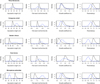 |
Fig. 1 Prior (dashed lines) and posterior density distributions (solid lines) of four parameters (L∞, k, t0, and p) for all five species for the G-VBGM model. |
Deviance information criterion (DIC) values for the four growth models (G-VBGM, SRGM, GGM and VBGM) used in this study.
Log pointwise predictive density (lppdLOOCV) and expected log predictive density for a new data point (elpdDIC) for four growth models (G-VBGM, SRGM, GGM and VBGM). Bold values indicate the model with the smallest values.
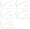 |
Fig. 2 Variations in leave-one-out (a) and smooth leave-one-out (b) errors as a function of log(λ 2) for Micropterus salmoides. |
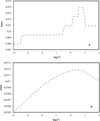 |
Fig. 3 (a) Growth rates (dL/dt) of Sander vitreus in relation to age group estimated by each model; (b) Growth rates (dL/dt) for Sander vitreus in relation to length estimated by each model. |
4 Discussion
4.1 Selection of growth models
Environmental change can affect the growth of individual fish and their age at maturity, so validated ages and growth estimates are important in fisheries studies (Essington et al., 2001; Cailliet et al., 2006; Haddon 2010; Froese et al., 2014). Previous investigations on marine fishes have demonstrated GGM to be best-suited for yellowfin tuna Thunnus albacares (Quinn and Deriso, 1999), G-VBGM for swordfish Xiphias gladius, and SRGM for rougheye rockfish Sebastes aleutianus (Soriano et al., 1992; Katsanevakis, 2006). In this study when we fitted VBGM, GGM, SRGM and G-VBGM to length-at-age datasets, large model-dependent differences in estimated growth parameters and growth rates were evident. Using DIC values, GGM was selected for one species (C. artedi) and G-VBGM for the other three. As an extended form of VBGM, G-VBGM considers the allocation of surplus energy to reproduction, and can jointly describe growth for adult and juvenile stages (Vrugt et al., 2009; Ohnishi et al., 2012). The G-VBGM applies the modified Richards equation (Tab. 2), which is promising to play an important role in fish-growth research as an extended form of the VBGM (Misra, 1986; Quinn and Deriso, 1999; Szalai et al., 2003; Katsanevakis, 2006). Overall performance results suggested that G-VBGM was the most reliable among the four candidate models for the four length-age datasets and the employed fitting method.
The underlying principle of the VBGM is that fish growth rate decreases in a linear manner with size (Katsanevakis, 2006; Haddon et al., 2008). Bustos et al. (2009) reported that VBGM did not properly describe growth over the first few years of life for cyprinids, while that this stage was better described by a GGM. The GGM assumes an exponential decrease in growth rate with size, compared to the sigmoidal growth curve, while the SRGM represents an omnibus approach for fitting fish growth (Quinn and Deriso, 1999; Katsanevakis, 2006).
4.2 Bayesian approach and the DIC
The Bayesian framework provides a way for directly estimating parameters and quantifying variance components and model parameter uncertainties (Gelman and Rubin, 1992). Thus it is more straightforward to calculate simultaneous credible intervals for multiple parameters, and to construct intervals around model predictions (Vrugt et al., 2009; Haddon, 2010). Through Bayesian analysis, we can analyze the role of alternative information sources in support of decision-making, and the effects of alternative decisions on various conservation or management aims (Gelman and Rubin, 1992; Cowles and Carlin, 1996; Brooks and Roberts, 1998; Vrugt et al., 2009; Kuikka et al., 2014). Bayesian statistics have considerably advanced fisheries analyses. A main advantage of Bayesian methods is that posterior inference is quite straightforward using MCMC outputs, because methods provide direct samples of posterior distributions of parameters of interest (Gelman and Rubin, 1992; Cowles and Carlin, 1996; O'Hara and Sillanpää, 2009).
Model performance was evaluated using DIC in stochastic Bayesian statistics, which incorporates the likelihood to generate posterior estimates of model parameters (Carlin and Louis, 2009; Zhu et al., 2016). Listed in ascending order of DIC values for P. flavescens, the G-VBGM model had the smallest DIC (259.51), with SRGM the next most plausible model (ΔDIC = 5.68). The GGM and VBGM models had DIC values of 285.72 (with ΔDIC, 26.21) and 282.92 (with ΔDIC, 23.41), respectively, and were generally intermediate to all the species growth examined. Spiegelhalter et al., (2002) reported that informative priors influence the results of both model parameters and DIC values (Spiegelhalter et al., 2014). Application of the DIC continues to be controversial among statisticians, because no unique driving principle for constructing DICs exists (Helser and Lai, 2004; Vrugt et al., 2009; Jiao et al., 2010; Spiegelhalter et al., 2014; Tang et al., 2014). The choice of a criterion of fit should depend on the objectives of the model (Brooks and Roberts, 1998; Cailliet et al., 2006; Katsanevakis and Maravelias, 2008; Haddon, 2010).
4.3 Uncertainty
To examine model uncertainty apart from checking the performances of growth functions based on DIC, the model evaluation method given by the LOOCV error was developed. A sensitivity index summarizes the elasticity of a variable with respect to a parameter (Pannell 1997; Pardo et al., 2018). The greater the elasticity, the higher the sensitivity of results to changes in a parameter. We used the LOOCV-based generalization error estimator as the performance evaluation criterion for model selection. For performance evaluation purposes, unbiased estimators and a low-variance regime are required for a model (Bo et al., 2006; Gelman et al., 2014). The LOOCV is the most classic exhaustive cross-validation procedure (Arlot and Celisse, 2010). Under the smoothness conditions on density, the smoothed LOOCV yielded excellent asymptotic model-selection performances, proving its asymptotic optimality (Langaas et al., 2005). Combining both the DIC and LOOCV provided a robust approach to model-selection uncertainty analysis. Based on estimates given by Bayesian LOOCV, the G-VBGM had the best predictive ability for the five freshwater fish species datasets.
In conclusion, we recommend fish growth models other than VBGM should be considered. For the five fish species examined, the VBGM did not properly describe growth during the first few years of life (Fig. 4). The alternative GGM assumes an exponential decrease in growth rate with size while the SRGM provides an omnibus approach for modelling fish growth. For checking model performance, DIC and LOOCV proved useful.
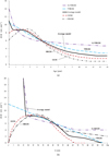 |
Fig. 4 The length at age data (dots) of the five fish species and the fitted curves for the four growth models (G-VBGM, SRGM, GGM and VBGM) used in this study. |
Acknowledgements
The authors thank Drs Yan Jiao, Xiujuan Shan, and Lisha Guan for sharing their expertise on the research. Specifically, we thank Drs Qun Liu, Jacob Johansen, Natalie Korszniak, and Andrew Bullen for their assistance on earlier drafts of the manuscript. We appreciate valuable comments made by Dr. Verena Trenkel, and three anonymous reviewers, which significantly improved our manuscript. This research was supported in part by the National Key R&D Program of China (grant no. 2018YFD0900906 and 2017YFE0104400), and Shandong Provincial Natural Science Foundation (grant no. ZR201702060096).
References
- Arlot S, Celisse A. 2010. A survey of cross-validation procedures for model selection. Statist Surv 4: 40–79. [CrossRef] [MathSciNet] [Google Scholar]
- Bo L, Wang L, Jiao L. 2006. Feature scaling for kernel fisher discriminant analysis using leave-one-out cross validation. Neural Comput 18: 961–978. [Google Scholar]
- Brooks SP, Roberts GO. 1998. Convergence assessment techniques for Markov chain Monte Carlo. Stat Comput 8: 319–335. [Google Scholar]
- Brosse S, Beauchard O, Blanchet S, Dürr HH, Grenouillet G, Hugueny B, Oberdorff T. 2013. Fish-SPRICH: a database of freshwater fish species richness throughout the World. Hydrobiologia 700: 343–349. [Google Scholar]
- Bustos R, Luque Á, Pajuelo JG. 2009. Age estimation and growth pattern of the island grouper, Mycteroperca fusca (Serranidae) in an island population on the northwest coast of Africa. Sci Mar 73: 319–328. [CrossRef] [Google Scholar]
- Cailliet GM, Smith WD, Mollet HF, Goldman KJ. 2006. Age and growth studies of chondrichthyan fishes: the need for consistency in terminology, verification, validation, and growth function fitting. Environ Biol Fish 77: 211–228. [CrossRef] [Google Scholar]
- Carlin BP, Louis TA. Bayesian Methods for Data Analysis. 3rd edn, CPC Press, Boca Raton, 2009. [Google Scholar]
- Chen Y, Jiao Y, Chen L. 2003. Developing robust frequentist and Bayesian fish stock assessment methods. Fish Fish 4: 105–120. [CrossRef] [Google Scholar]
- Cowles MK, Carlin BP. 1996. Markov chain Monte Carlo convergence diagnostics: a comparative review. J Am Stat Assoc 91: 883–904. [Google Scholar]
- Eastwood S, Couture P. 2002. Seasonal variations in condition and liver metal concentrations of Yellow Perch (Perca flavescens) from a metal-contaminated environment. Aquat Toxicol 58: 43–56. [CrossRef] [PubMed] [Google Scholar]
- Essington TE, Kitchell JF, Walters CJ. 2001. The von Bertalanffy growth function, bioenergetics, and the consumption rates of fish. Can J Fish Aquat Sci 58: 2129–2138. [Google Scholar]
- Froese R, Thorson JT, Reyes RB. 2014. A Bayesian approach for estimating length-weight relationships in fishes. J Appl Ichthyol 30: 78–85. [Google Scholar]
- Gelman A, Hwang J, Vehtari A. 2014. Understanding predictive information criteria for Bayesian models. Stat Comput 24: 997–1016. [Google Scholar]
- Gelman A, Rubin DB. 1992. Inference from iterative simulation using multiple sequences. Stat Sci 21: 457–472. [Google Scholar]
- Gompertz B. 1825. On the nature of the function expressive of the law of human mortality, and on a new mode of determining the value of life contingencies. Phil Trans of the Royal Soc 182: 513–585. [Google Scholar]
- Haddon M. Modelling and Quantitative Methods in Fisheries . 2nd edn, Chapman and Hall, New York, 2010. [Google Scholar]
- Haddon M, Mundy C, Tarbath D. 2008. Using an inverse-logistic model to describe growth increments of blacklip abalone (Haliotis rubra) in Tasmania. FISH B-NOAA 106: 58–71. [Google Scholar]
- He JX, Rudstam LG, Forney JL, VanDeValk AJ, Stewart DJ. 2005. Long-term patterns in growth of Oneida Lake Walleye: a multivariate and stage-explicit approach for applying the von Bertalanffy growth function. J Fish Biol 66: 1459–1470. [Google Scholar]
- Helser TE, Lai HL. 2004. A Bayesian hierarchical meta-analysis of fish growth: with an example for North American Largemouth Bass, Micropterus salmoides . Ecol Model 178: 399–416. [CrossRef] [Google Scholar]
- Heyer CJ, Miller TJ, Binkowski FP, Caldarone EM, Rice JA. 2001. Maternal effects as a recruitment mechanism in Lake Michigan Yellow Perch (Perca flavescens). Can J Fish Aquat Sci 58: 1477–1487. [Google Scholar]
- Jessop BM. 2010. Geographic effects on American eel (Anguilla rostrata) life history characteristics and strategies. Can J Fish Aquat Sci 67: 326–346. [Google Scholar]
- Jiao Y, Neves R, Jones J. 2008. Models and model selection uncertainty in estimating growth rates of endangered freshwater mussel populations. Can J Fish Aquat Sci 65: 2389–2398. [Google Scholar]
- Jiao Y, Reid K, Nudds T. 2006. Variation in the catchability of Yellow Perch (Perca flavescens) in the fisheries of Lake Erie using a Bayesian error-in-variable approach. ICES J Mar Sci 63: 1695–1704. [Google Scholar]
- Jiao Y, Reid K, Nudds T. 2010. Consideration of uncertainty in the design and use of harvest control rules. Sci Mar 74: 371–384. [CrossRef] [Google Scholar]
- Jonsson B, Jonsson N. 2009. A review of the likely effects of climate change on anadromous Atlantic salmon Salmo salar and brown trout Salmo trutta, with particular reference to water temperature and flow. J Fish Biol 75: 2381–2447. [PubMed] [Google Scholar]
- Kang B, Deng J, Wu Y, Chen L, Zhang J, Qiu H, He D. 2014. Mapping China's freshwater fishes: diversity and biogeography. Fish Fish 15: 209–230. [CrossRef] [Google Scholar]
- Katsanevakis S. 2006. Modelling fish growth: model selection, multi-model inference and model selection uncertainty. Fish Res 81: 229–235. [Google Scholar]
- Katsanevakis S, Maravelias CD. 2008. Modelling fish growth: multi-model inference as a better alternative to a priori using von Bertalanffy equation. Fish Fish 9: 178–187. [CrossRef] [Google Scholar]
- Kimura DK. 1980. Likelihood methods for the von Bertalanffy growth curve. Fisheries Bulletin 77: 765–774. [Google Scholar]
- Kuikka S, Vanhatalo J, Pulkkinen H, Mäntyniemi S, Corander J. 2014. Experiences in Bayesian inference in Baltic Salmon management. Stati Sci 29: 42–49. [MathSciNet] [Google Scholar]
- Langaas M, Lindqvist BH, Ferkingstad E. 2005. Estimating the proportion of true null hypotheses, with application to DNA microarray data. J R Stat Soc B 67: 555–572. [CrossRef] [MathSciNet] [Google Scholar]
- Liu C, Wan R, Jiao Y. 2017. Exploring non-stationary and scale-dependent relationships between walleye (Sander vitreus) distribution and habitat variables in Lake Erie. Mar Freshwater Res 68: 270–281. [CrossRef] [Google Scholar]
- Michielsens CG, McAllister MK. 2004. A Bayesian hierarchical analysis of stock recruit data: quantifying structural and parameter uncertainties. Can J Fish Aquat Sci 61: 1032–1047. [Google Scholar]
- Misra R.K. 1986. Fitting and comparing several growth curves of the generalized von Bertalanffy type. Can J Fish Aquat Sci 43: 1656–1659. [Google Scholar]
- Nylander JA, Wilgenbusch JC, Warren DL, Swofford DL. 2008. AWTY (are we there yet?): a system for graphical exploration of MCMC convergence in Bayesian phylogenetics. Bioinformatics 24: 581–583. [CrossRef] [PubMed] [Google Scholar]
- O'Hara RB, Sillanpää MJ. 2009. A review of Bayesian variable selection methods: what, how and which. Bayesian Anal 4: 85–117. [Google Scholar]
- Ohnishi S, Yamakawa T, Okamura H, Akamine T. 2012. A note on the von Bertalanffy growth function concerning the allocation of surplus energy to reproduction. Fish B-NOAA 110: 223–229. [Google Scholar]
- Panhwar SK. Some aspects of fish population dynamics of the commercial fish species in Pakistan. PhD Thesis. Ocean University of China, Qingdao, 2012. [Google Scholar]
- Pannell DJ. 1997. Sensitivity analysis: strategies, methods, concepts, examples. Agric Econ 16: 139–152. [Google Scholar]
- Pardo SA, Cooper AB, Reynolds JD, Dulvy NK. 2018. Quantifying the known unknowns: estimating maximum intrinsic rate of population increase in the face of uncertainty. ICES J Mar Sci 75: 953–963. [Google Scholar]
- Pilling GM, Kirkwood GP, Walker SG. 2002. An improved method for estimating individual growth variability in fish, and the correlation between von Bertalanffy growth parameters. Can J Fish Aquat Sci 59: 424–432. [Google Scholar]
- Quinn TJ, Deriso RB. Quantitative Fish Dynamics . 1st edn, Oxford University Press, Oxford, 1999. [Google Scholar]
- Román-Román P, Romero D, Torres-Ruiz F. 2010. A diffusion process to model generalized von Bertalanffy growth patterns: Fitting to real data. J Theor Biol 263: 59–69. [CrossRef] [MathSciNet] [PubMed] [Google Scholar]
- Schneider JC. Manual of fisheries survey methods II: with periodic updates. Michigan Department of Natural Resources, Fisheries Special Report 25, Michigan, USA, 2000. [Google Scholar]
- Schnute J, Richards LJ. 1990. A unified approach to the analysis of fish growth, maturity, and survivorship data. Can J Fish Aquat Sci 47: 24–40. [Google Scholar]
- Soriano M, Moreau J, Hoenig JM, Pauly D. 1992. New functions for the analysis of two-phase growth of juvenile and adult fishes, with application to Nile Perch. T Am Fish Soc 121: 486–493. [CrossRef] [Google Scholar]
- Stockwell JD, Yule DL, Gorman OT, Isaac EJ, Moore SA. 2006. Evaluation of bottom trawls as compared to acoustics to assess adult Lake Herring (Coregonus artedi) abundance in Lake Superior. J Great Lakes Res 32: 280–292. [Google Scholar]
- Spiegelhalter DJ, Best NG, Carlin BP, Linde A. 2014. The deviance information criterion: 12 years on. J R Stat Soc B 76: 485–493. [CrossRef] [MathSciNet] [Google Scholar]
- Spiegelhalter DJ, Best NG, Carlin BP, Van Der Linde A. 2002. Bayesian measures of model complexity and fit. J R Stat Soc B 64: 583–639. [CrossRef] [MathSciNet] [Google Scholar]
- Szalai EB, Fleischer GW, Bence JR. 2003. Modelling time-varying growth using a generalized von Bertalanffy model with application to bloater (Coregonus hoyi) growth dynamics in Lake Michigan. Can J Fish Aquat Sci 60: 55–66. [Google Scholar]
- Tang M, Jiao Y, Jones JW. 2014. A hierarchical Bayesian approach for estimating freshwater mussel growth based on tag-recapture data. Fish Res 149: 24–32. [Google Scholar]
- Vilizzi L, Copp GH. 2017. Global patterns and clines in the growth of common carp Cyprinus carpio . J Fish Biol 91: 3–40. [CrossRef] [PubMed] [Google Scholar]
- Vrugt JA, Ter Braak CJ, Gupta HV, Robinson BA. 2009. Equifinality of formal (DREAM) and informal (GLUE) Bayesian approaches in hydrologic modelling? Stoch Env Res Risk A 23: 1011–1026. [CrossRef] [Google Scholar]
- Wilberg MJ, Bence JR. 2008. Performance of deviance information criterion model selection in statistical catch-at-age analysis. Fish Res 93: 212–221. [Google Scholar]
- Zhu X, Tallman RF, Howland KL, Carmichael TJ. 2016. Modeling spatiotemporal variabilities of length-at-age growth characteristics for slow-growing subarctic populations of Lake Whitefish, using hierarchical Bayesian statistics. J Great Lakes Res 42: 308–318. [Google Scholar]
- Zellner A. 1971. Bayesian and non-bayesian analysis of the log-normal distribution and log-normal regression. J Am Stat Assoc 66: 327–330. [Google Scholar]
Cite this article as: Zhang K, Zhang J, Li J, Liao B,. 2020. Model selection for fish growth patterns based on a Bayesian approach: A case study of five freshwater fish species. Aquat. Living Resour. 33: 17
All Tables
Mean total length (cm) and standard deviations (in brackets) by age group and number of observations for five freshwater fish species.
Functions of the four growth models (VBGM, GGM, SRGM, G-VBGM) used in this study.
Mean and standard deviations (SD) for lognormal prior distributions used for asymptotic length (L∞) for five freshwater fish used in Bayesian analysis.
Posterior means and 95% credible intervals [in brackets] of the parameters of four growth models (G-VBGM, GGM, VBGM and SRGM) fitted to mean length-at-age data for five fish species.
Deviance information criterion (DIC) values for the four growth models (G-VBGM, SRGM, GGM and VBGM) used in this study.
Log pointwise predictive density (lppdLOOCV) and expected log predictive density for a new data point (elpdDIC) for four growth models (G-VBGM, SRGM, GGM and VBGM). Bold values indicate the model with the smallest values.
All Figures
|
Fig. 1 Prior (dashed lines) and posterior density distributions (solid lines) of four parameters (L∞, k, t0, and p) for all five species for the G-VBGM model. |
| In the text | |
|
Fig. 2 Variations in leave-one-out (a) and smooth leave-one-out (b) errors as a function of log(λ 2) for Micropterus salmoides. |
| In the text | |
|
Fig. 3 (a) Growth rates (dL/dt) of Sander vitreus in relation to age group estimated by each model; (b) Growth rates (dL/dt) for Sander vitreus in relation to length estimated by each model. |
| In the text | |
|
Fig. 4 The length at age data (dots) of the five fish species and the fitted curves for the four growth models (G-VBGM, SRGM, GGM and VBGM) used in this study. |
| In the text | |
Current usage metrics show cumulative count of Article Views (full-text article views including HTML views, PDF and ePub downloads, according to the available data) and Abstracts Views on Vision4Press platform.
Data correspond to usage on the plateform after 2015. The current usage metrics is available 48-96 hours after online publication and is updated daily on week days.
Initial download of the metrics may take a while.